Identification of habitat requirements of farmland birds based on a hierarchical structured monitoring scheme

Introduction

Of a total of approximately 10000 bird species, about 3600 are considered farmland birds (Weijden et al., 2010). In terms of bird diversity this is the second largest 'group' after forest and scrubland birds. However, rather than applying to a single systematic group, the widely-used term 'farmland bird' is loosely applied to any bird species either breeding or regularly foraging in agricultural areas.

In Europe, approximately 330 species are considered 'farmland birds' whereas in Asia, approximately 1300 species are assigned to this group (Weijden et al., 2010). Farmland can be classified into different types but in terms of bird diversity, extensively used arable land, in-terspersed with seminatural habitats and fallows is the richest farmland habitat type (Oppermann et al., 2012). Within these landscapes, areas exhibiting different land use types and structural diversity are particularly species-rich (Hoffmann et al., 2000; Oppermann and Hoffmann, 2012). However, many recent studies have demonstrated a strong decline in bird species diversity as agriculture has intensified and crop diversity has been reduced (e.g. Chamberlain et al., 2000; Newton, 2004; Donald et al., 2006; Wretenberg et al., 2006; Geiger et al., 2010).

A clear indication of a general decline in farmland bird abundances is given by the bird indicators of the European Union and individual European countries. These farmland bird indicators are also considered to be indicators of biodiversity in general (e.g. PECBMS, 2009; EEA, 2010; Sudfeldt et al., 2010). Most bird species indices are currently based on monitoring data for selected indicator bird species, recorded on plots of 1 km² size and collected annually for several years in the same area on a country or European scale. These indicators are important for the assessment of biodiversity and currently show low values and a continuing negative trend over the last 20 years.

In the context of the aims of the Convention on Biological Diversity (CBD) a continuing loss of biodiversity should be avoided and biodiversity supporting activities must be established. In Europe a new biodiversity strategy has been developed (COM, 2011), in which the conservation and advancement of biodiversity in agrarian regions is especially emphasized.

In Germany, the national bird indicator for "Species Diversity and Landscape Quality" (Sudfeldt et al., 2010) is a dimensionless population index and has a weak relation to potentially suitable habitat parameters for the given landscape. This indicator does not therefore provide any information on the potential effects of different field crops, vegetation structure or other habitats on the habitat suitability for breeding birds. Each of these parameters may affect individual species and/or local populations and therefore entire species diversity on the landscape scale. These information gaps are also present in the European farmland bird index (PECBMS, 2009). Additionally, there is currently insufficient information concerning the positive and negative influences of agricultural land use on bird indices. Accordingly, existing bird indicators cannot be readily used for the formulation of biodiversity conservation strategies. Methods are therefore needed which combine bird abundance data in farmlands with habitat and land use parameters. This combination would allow the identification of habitat suitability characteristics for farmland bird species in order to support and protect bird species diversity in agricultural landscapes. An approach such as this should reflect heterogeneity of site conditions within agricultural landscapes as well as the specific suitability of different crops and other habitats, e.g. seminatural biotopes. Thus, it should be possible to quantify the habitat preferences of the bird species investigated. The aim of this study was to design and test a suitable monitoring scheme for farmland birds which allows detailed analyses and information of the bird species requirements in relation to agricultural land use and habitat availability on different spatial scales.

Methods

Study area

The study area was located in north eastern Germany (Federal State of Brandenburg), in the counties Märkisch-Oderland, Barnim and Uckermark. The mean annual temperature of the region is 8.4℃, with mean annual precipitation of 520 mm. Approximately half of the land surface is used for agriculture, mainly as arable land, with winter wheat, winter rape and maize as the most abundant crops. Field sizes in the study area vary largely, from < 0.5 ha to 97 ha, with approximately 50% between 3 and 30 ha. The average field size area is 19.3 ha. Approximately 5% to 7% of the landscape comprising the study area is covered by seminatural habitats and structures, e.g. small woodlands, water bodies and field margins.

Selection and size of the study plots

For statistically sound data analysis and overall representative results, the size of the investigation area is critical, and often neglected in small scale investigations dealing with species abundances and the associated reasoning. In Germany, bird monitoring programs are usually conducted on plots of 100 ha (= 1 km²) (for the national monitoring program including many agricultural areas see Sudfeldt et al., 2012). In order to gain sufficient information about the abundances of bird species in farmland (i.e. the number of territories per 10 ha) the design of the current study was based on preliminary field work (Hoffmann and Kiesel, 2007, Hoffmann et al. 2007). The aim was to obtain baseline data on all bird species occurring in the region and the variability in their abundances. This information was used to determine the number of plots and the total area for the entire monitoring project. The main criterion for the number and the total area of the study plots was the average area needed for the detection of one breeding bird territory of each species — the 'single territory detection area' (STDA). STDA is defined as the average size of an area (ha) within an agricultural landscape needed to detect a territory of a breeding bird species (Hoffmann and Kiesel, 2007, 2009; Table 1). Consequently, to ensure that the sample size for the most frequent species was adequate for statistical analysis and also to detect the less frequent farmland species, 29 individual 1 km² study plots were selected for the bird surveys.

Table  1.  Single territory detection area (STDA) for ten farmland bird species with various abundances in agricultural landscapes of the Federal State of Brandenburg, Germany, based on Hoffmann and Kiesel (2007).

Bird species	STDA (ha)
Skylark (Alauda arvensis)	5
Yellowhammer (Emberiza citrinella)	21
Yellow Wagtail (Motacilla flava)	29
Corn Bunting (Emberiza calandra)	43
Whitethroat (Sylvia communis)	58
Red-backed Shrike (Lanius collurio)	80
Tree Sparrow (Passer montanus)	97
Whinchat (Saxicola rubetra)	135
Common Quail (Coturnix coturnix)	232
Grey Partridge (Perdix perdix)	2167

 | Show Table

DownLoad: CSV

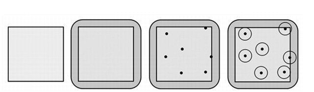
In order to analyze all the data collected and to include bird territories on the edges of the sampling plots, a 100 m buffer zone was included around the 1 km² plots. This resulted in a total area of 1.43 km² per plot (Fig. 1). These plots were carefully mapped with respect to land use, habitat types and vegetation structures in each of the eight surveys per plot and year.

Figure  1.  Design of the monitoring plots from left to right: bird survey area (1 km²), land use survey area (1.43 km²), example of territory points (TPs) of breeding birds, and circular areas around the TPs.

DownLoad: Full-Size Img PowerPoint

The exact location of each study plot was determined using aerial photographs and land use maps (provided by the respective farmers/land owners). In order to assess the effect of the dominating crops (winter wheat, winter rape and maize) on bird occurrence, we selected three sets of seven plots each in which the respective crop covered more than 50% of the area (plus other crops and seminatural habitats). Seven more plots were dominated by 'self greened fallow land' (fallow land). Additionally, one plot was available in which fallow land was converted into arable land. In contrast to typical crop fields, the vegetation of fallow land is characterized by spontaneous secondary succession. This vegetation type was abundant in the past, however it decreased dramatically in course of land use intensification after the EU subsidies were cut in 2007. In total, 29 plots of 1 km² were investigated for the bird survey and extended to 1.43 km² size each for the survey of land use and habitats (Fig. 1).

Finally, GIS-based data processing and evaluations were conducted using ArcGIS (program ArcInfo 9.3). The maps for the field work were based on this information, and the data base was used for all subsequent data processing.

Bird surveys

The bird surveys were conducted 2009 and 2010 using the territory mapping method described by Dornbusch (1968), Oelke et al. (1968), Fischer et al. (2005) and Hoffmann et al. (2012). In contrast to methods such as point counts or line and transect mapping (frequently applied in bird monitoring programs) territory mapping covers almost completely the whole monitoring plot. Because of this 'spatially completeness', this method is particularly suitable for spatial analysis connecting bird data with land use and habitat variables.

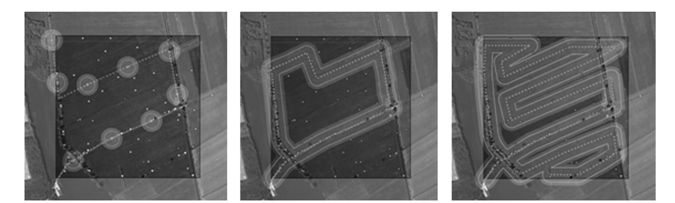
The pathways of each field worker during the surveys were determined according to the actual habitat distribution within the plots and were attempted to cover the entire plot area (Fig. 2). In order to record the temporal abundance of breeding bird species throughout the whole season, the surveys started in the second half of March when sedentary bird species begin their territorial activities and the first migratory farmland species arrive in the study area. The plots were monitored until the breeding season for farmland bird species was almost finished, i.e. the middle of July. We defined 'breeding season' as the time period in which territorial behavior of birds could be observed.

Figure  2.  Comparison of the three common field methods for recording bird abundances: left – 'point counts', middle – 'line mapping', right – 'territory mapping'. Dots: territory points of breeding birds; dotted line: inspection route of the observer; light gray area: monitored area by the observer (50 to 75 m wide).With increasing coverage the proportion of the detected TPs increases, and the spatial scale of habitat distribution and land use patterns becomes more easily quantifiable.

DownLoad: Full-Size Img PowerPoint

In 2009 five field surveys were conducted between mid-March and mid-June. This was expanded to eight surveys, mid-March until the end of July in 2010 to cover the entire breeding season of all migrating bird species. The surveys were conducted in two-weekly intervals. During the surveys, the territorial characteristics of the birds, especially singing males, were noted and mapped (Südbeck et al., 2005; Hoffmann et al., 2012). The location of each singing male was mapped as accurately as possible as point information ('territory point' — TP) in the map (Fig. 1) of the plot. Our intention was to survey each plot for 2–3 hours. The mean duration of the surveys was 230 minutes (min. 160, max. 300). The complete annual data for each TP of the bird species for each plot consisted of eight maps and protocols, which were fed into a GIS database as point shapes. This database was then used to describe bird species diversity and abundances (territories per 10 ha) and to relate the bird data to habitat characteristics on various spatial scales.

Mapping of the arable fields and habitats

The exact distribution and locations of arable fields was based on aerial photographs and (when available) on field maps provided by the respective farmers. Before the start of the field investigations, the shapes of each arable field were digitized and saved in a GIS-based databank as area shapes, in which each plot and each field were given an ID. Because even during the growth period the spatial arrangement of arable crops was dynamic to some extent, e.g. due to reseeding, the actual location of each arable field was checked during each of the eight field surveys per year and adjusted if different from the prepared map. All other habitats, e.g. seminatural habitats and anthropogenic habitats such as paths, roads and settlements were also mapped (Fig. 1). A numerical habitat code was assigned to each habitat type. In this way, in order to provide detailed characteristics of the habitat types a total of 41.5 km² was mapped five times in 2009 and eight times in 2010.

Mapping of field crops and vegetation structures

The crops and vegetation structures present on each of the study plots were mapped during the field surveys. In this way precise information was obtained on the spatial distribution of crops and the development of vegetation structural characteristics throughout the breeding bird monitoring period.

Vegetation structure is particularly important for the suitability of agricultural areas for farmland birds. However, vegetation structural parameters for different crops vary greatly throughout their respective growth periods resulting in differences in the suitability of various areas for farmland birds. We therefore distinguished three structural variables and classified each crop field according to: ⅰ) plant height; ⅱ) vegetation coverage; and ⅲ) vegetation density. Four classes for each of these parameters were assigned (Table 2). While vegetation height and coverage were estimated visually, vegetation density was defined as a variable indicating the combination of the parameters height and density as the architectural complexity of the vegetation layer (Table 3). Table 2 summarizes the parameters and classes, which were used for each individual crop field in each survey. However, rather than being a simple function of height and coverage, crop density is indicative of the complex three dimensional arrangement of plant structures. In the current study, field workers assigned individual crop fields to density classes according to the assessment scheme shown in Table 3. These data were fed into the same data base as the bird data.

Table  2.  Classification scheme for vegetation structure: height, coverage and density as applied on each crop field at each survey

Variables	Classes
Vegetation height (m)	0–0.25	> 0.25–0.5	> 0.5–0.75	> 0.75
Vegetation coverage (%)	0–25	> 25–50	> 50–75	> 75
Vegetation density	low	medium	high	very high

 | Show Table

DownLoad: CSV

Table  3.  Vegetation density classes (l — low, m — medium, h — high, vh — very high) in relation to plant height and coverage, the assignments are variable depending on the physical arrangement of the plant structures

Height (m)	Coverage (%)
	0–25	> 25–50	> 50–75	> 75
0–0.25	l	l or m	m	m or h
> 0.25–0.5	l	m	m or h	h
> 0.5–0.75	m	m	h	h or vh
> 0.75	m	m or h	h	vh

 | Show Table

DownLoad: CSV

Habitat matrix of breeding birds

Birds recognize potential breeding territories within the utilized landscape. Thus, individual birds select those areas within a landscape which seem suitable for breeding, foraging and provisioning their young. Bird territories are therefore located within those parts of the landscape with the most favorable spatial configurations for the respective species. In order to determine the habitat preferences of individual species, a species-specific analysis of habitat configurations within the breeding territories was conducted. The area around each TP within a radius of 100 m (3.14 ha) was analyzed, in line with literature data of breeding territory sizes of about 0.5 to 3.0 ha for most passerine farmland bird species (Bauer et al., 2005).

This habitat configuration of the circular area around each TP was defined as 'habitat matrix' (HM). Because the monitoring plots of 1 km² were buffered by a 100 m zone (in total 1.43 km²), the HM of all TPs within the plots could be analyzed completely and without any edge effect (Fig. 1). For the identification of potential differences within the area around each TP, the radius of the circle was increased stepwise from 10 to 100 m, with increments of 10 m. The smallest HM therefore was 314 m² (r = 10 m) and the largest 31400 m² (r = 100 m). The descriptions of these circular territories were made for each of the 13 field surveys for each TP of the bird species. The resulting HMs were then analyzed with GIS, using SAS statistical software and the JUMP program block as described by Bradley and Sall (2011).

Results

Hierarchical structure of the data

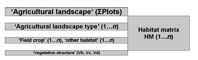
The data collection methodology was designed to 'zoom in' from the landscape scale into the vegetation structure of bird territories and infer species-specific habitat characteristics from spatial information. Accordingly, the data were hierarchically structured and analyzed (Fig. 3).

Figure  3.  Hierarchical structure of the data collection scheme with options for data analysis on different spatial scales — the agricultural landscape, agricultural landscape types, field crops and other habitats, and vegetation structure height (Vh), coverage (Vc), and density (Vd) of the crops and the habitat matrix (HM).

DownLoad: Full-Size Img PowerPoint

The largest spatial scale of analysis, in which all data of all plots are summarized, is the agricultural landscape. Central European agricultural landscapes are typically composed of a 'main land use type', dominated by a specific crop. Four land use types were predominant in the study area, the dominating crops being winter wheat, winter rape, maize and fallow land. Each of these land use types was represented by seven plots, which allowed specific analyses of farmland bird occurrence within various typical land use patterns. On the spatial scale 'field crops and other habitats', the relation of bird occurrence to the geometry and spatial configuration of crop fields and other habitat types can be described and analyzed. On the next smaller scale, the vegetation parameters characterize the structure of the field crop vegetation, and their temporal changes of the structure throughout the growing period. In relation to the occurrence of farmland bird species the effects of the crop vegetation development on the habitat preferences of birds can be identified. Finally, the HM integrates the different spatial scales to identify territory information as species-specific spatial habitat prerequisites during the breeding season. The HM-concept allows the types and areas of all crops and other habitats investigated and their areas within the territories of individual birds and on species level to be quantified.

Areas of crop fields and habitats

The areas occupied by various crops and the areas of other habitats are summarized on the scale of the agricultural landscape in Table 4. In both years of the study the dominating crops were winter wheat, winter rape and maize which covered 65.3% (2009) and 67.9% (2010) of the total bird survey area. Fallow land occupied 14.1% (2009) and 11.6% (2010). Eighteen other crops were also grown in the area, representing 16.2% (2009) and 14.3% (2010) of the area, while all other habitats covered approximately 5% of the study area in both years (Table 4).

Table  4.  Proportion of crops and other habitats (ha and %) in the study area of 29 km² bird monitoring plots

Year	Crops															Other habitats
	Winter wheat			Winter rape			Maize			Fallow land			Other crops			Wood land			Grassland			Small water bodies			Roads, field paths			Settlement areas			Bogs/swamps
	ha	%		ha	%		ha	%		ha	%		ha	%		ha	%		ha	%		ha	%		ha	%		ha	%		ha	%
2009	755	26.0		645	22.2		496	17.1		407	14.1		470	16.2		51.7	1.8		33.5	1.2		24.5	0.8		9.1	0.3		5.2	0.2		3.3	0.1
2010	609	21.0		689	23.8		649	23.1		337	11.6		415	14.3		51.4	1.8		31.5	1.2		29.0	1.0		7.2	0.25		14.5	0.5		5.6	0.2

 | Show Table

DownLoad: CSV

Species diversity and abundance on the 'agricultural landscape'-scale

A total of 103 bird species with territorial behavior were detected, 39 (38%) of which are bird species typical of landscapes dominated by farmland areas, e.g. Skylark, Yellow Wagtail and Corn Bunting (Bauer et al., 2005). The temporal dynamics of detected abundances of these farmland bird species during the breeding season are shown in Table 5. As expected, the overall abundance, the time of maximum abundance and STDA varied between the species, e.g. the Skylark as the most frequent breeding bird species was most abundant in the second half of April, while the Corn Bunting was most abundant in May and first half of June. STDA varied extremely, between 3 ha for Skylark territories and 2900 ha for the Hoopoe (Upupa epops).

Table  5.  Temporal dynamics of abundances and 'single territory detection area' (STDA) of 38 farmland breeding bird species over the course of the breeding season in 2010. Species are listed in descending order of detected abundance.

Species	Abundance (territories per 100 ha)								STDA (ha)
	March 2	April 1	April 2	May 1	May 2	June 1	June 2	July 1
Skylark (Alauda arvensis)	23.76	28.48	30.00	27.24	24.55	23.52	21.31	16.34	3
Yellow Wagtail (Motacilla flava)	0.00	0.03	1.90	2.66	3.38	3.34	2.83	2.52	30
Corn Bunting (Emberiza calandra)	1.83	2.48	2.55	3.03	3.14	3.17	2.72	2.66	32
Marsh Warbler (Acrocephalus palustris)	0.00	0.00	0.00	0.21	1.72	2.62	2.00	1.45	38
Yellowhammer (Emberiza citrinella)	2.14	1.86	2.14	2.28	2.17	1.90	1.59	1.83	44
Whinchat (Saxicola rubetra)	0.00	0.00	0.24	1.24	1.72	1.66	1.24	0.55	58
Whitethroat (Sylvia communis)	0.00	0.00	0.34	1.10	1.07	1.24	0.97	0.93	81
Yellow Warbler (Hippolais icterina)	0.00	0.00	0.00	0.17	0.90	1.07	0.79	0.55	94
Red-backed Shrike (Lanius collurio)	0.00	0.00	0.00	0.24	0.79	1.03	0.97	0.93	97
Greenfinch (Carduelis chloris)	0.24	0.41	0.59	0.45	0.52	0.62	0.55	0.45	161
Tree Pipit (Anthus trivialis)	0.00	0.10	0.41	0.62	0.24	0.38	0.41	0.07	161
Tree Sparrow (Passer montanus)	0.21	0.48	0.66	0.48	0.59	0.52	0.31	0.17	171
Lesser Whitethroat (Sylvia currata)	0.00	0.07	0.34	0.52	0.34	0.14	0.21	0.10	193
Goldfinch (Carduelis carduelis)	0.14	0.31	0.17	0.48	0.31	0.24	0.28	0.31	207
Pheasant (Phasianus colchicus)	0.24	0.28	0.24	0.45	0.50	0.45	0.41	0.31	223
Woodlark (Lullula arborea)	0.28	0.28	0.10	0.07	0.14	0.03	0.21	0.00	363
Linnet (Carduelis cannabina)	0.10	0.10	0.14	0.03	0.14	0.21	0.10	0.07	483
Lapwing (Vanellus vanellus)	0.07	0.17	0.14	0.21	0.14	0.14	0.07	0.00	483
Crane (Grus grus)	0.14	0.21	0.03	0.07	0.03	0.03	0.03	0.00	483
Magpie (Pica pica)	0.17	0.10	0.14	0.10	0.07	0.07	0.03	0.03	580
Common Quail (Coturnix coturnix)	0.00	0.00	0.00	0.00	0.14	0.17	0.10	0.07	580
Marsh Harrier (Circus aeruginosus)	0.00	0.07	0.14	0.00	0.03	0.00	0.00	0.03	725
Ortolan Bunting (Emberiza hortulana)	0.00	0.00	0.00	0.03	0.03	0.07	0.03	0.00	725
Barn Swallow (Hirundo rustica)	0.00	0.03	0.00	0.14	0.14	0.00	0.03	0.03	725
Stonechat (Saxicola rubicola)	0.00	0.07	0.10	0.03	0.03	0.03	0.03	0.03	967
Greylag Goose (Anser anser)	0.10	0.07	0.00	0.00	0.03	0.00	0.00	0.00	967
Barred Warbler (Sylvia nisoria)	0.00	0.00	0.00	0.03	0.10	0.07	0.00	0.07	967
Northern Wheatear (Oenanthe oenanthe)	0.00	0.00	0.00	0.10	0.10	0.00	0.00	0.00	967
Meadow Pipit (Anthus pratensis)	0.00	0.07	0.07	0.03	0.00	0.03	0.00	0.00	1450
Grasshopper Warbler (Locustella naevia)	0.00	0.00	0.00	0.07	0.03	0.00	0.00	0.00	1450
Eurasian Buzzard (Buteo buteo)	0.03	0.00	0.00	0.00	0.00	0.00	0.00	0.00	2900
Crested Lark (Galerida cristata)	0.00	0.00	0.03	0.00	0.00	0.00	0.00	0.00	2900
Grey Partridge (Perdix perdix)	0.00	0.03	0.03	0.00	0.03	0.00	0.03	0.00	2900
Krestel (Falco tinnunculus)	0.00	0.00	0.03	0.03	0.00	0.00	0.00	0.00	2900
Little Ringed Plover (Charadrius dubius)	0.00	0.00	0.00	0.00	0.03	0.03	0.00	0.00	2900
Great Grey Shrike (Lanius excubitor)	0.03	0.00	0.00	0.00	0.00	0.00	0.00	0.00	2900
Turtle Dove (Streptopelia turtur)	0.00	0.00	0.00	0.03	0.00	0.03	0.00	0.07	2900
Hoopoe (Upupa epops)	0.00	0.00	0.00	0.00	0.03	0.00	0.00	0.00	2900

 | Show Table

DownLoad: CSV

Habitat requirements of farmland bird species on different spatial scales

The replicate bird territory mapping and simultaneous monitoring of habitat characteristics on different spatial scales allows identifying species specific relations of birds and landscape features. Three farmland bird species serve as examples: ⅰ) the abundances of the Corn Bunting on the spatial scales of the 'agricultural landscape, 'agricultural landscape types' and 'field crops'; ⅱ) the dynamic abundances of the Skylark in relation to different field crops and their vegetation structures in the course of the breeding season; and ⅲ) the habitat matrix analysis for Whinchat to compare the habitat configuration of the bird territories with the configuration of the landscape.

Abundance of the Corn Bunting on different spatial scales

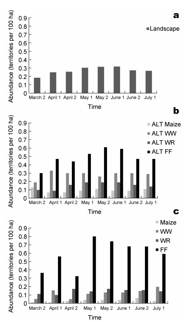
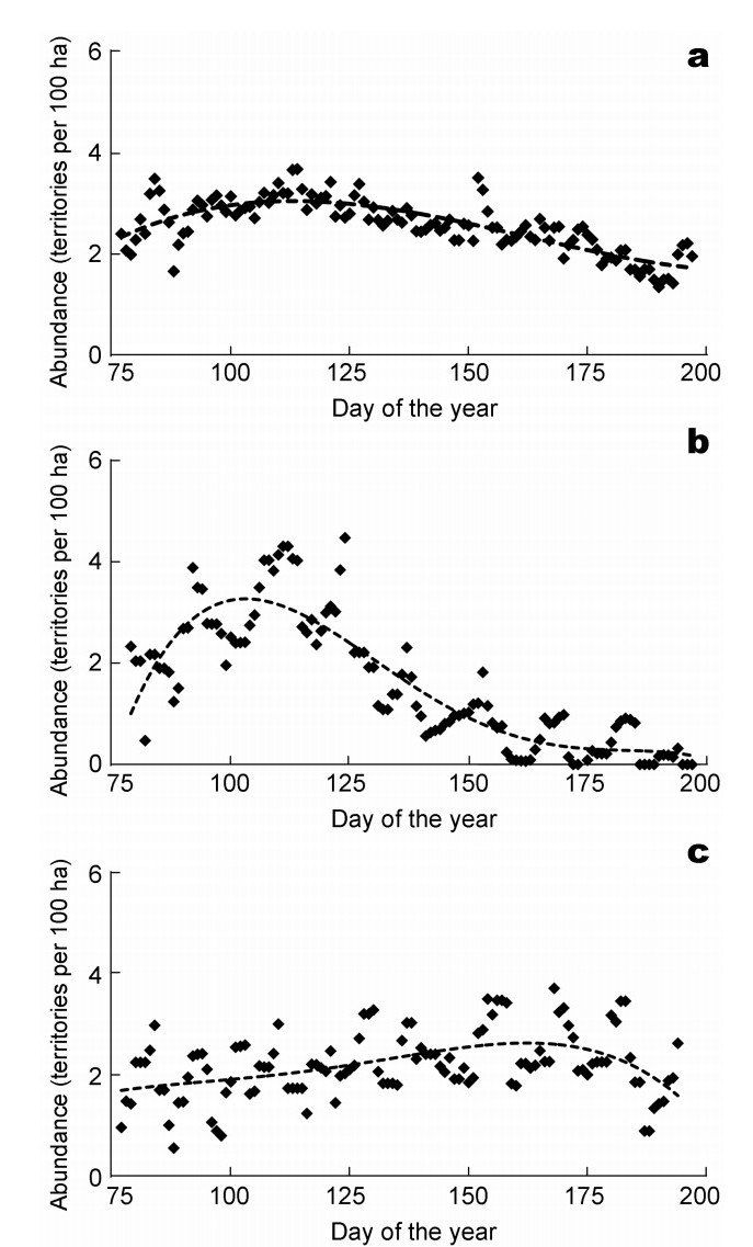
The Corn Bunting is a typical farmland bird and wide-spread throughout Europe (BirdLife, 2004). This species occupies territories in Germany in March, and its breeding period begins a few weeks later in early May (Fischer, 2003). On the 'agricultural landscape' scale, a maximum of 0.32 territories per 10 ha were detected during the main breeding period between early May and mid-June (Fig. 4, above). On the spatial scale of 'agricultural landscape type' it is obvious that different habitat types within the landscape have different importance for the Corn Bunting (Fig. 4, middle). In areas dominated by fallow land, the Corn Bunting had 0.48 to 0.61 territories per 10 ha during the main breeding period. In maize-dominated areas, only about 0.10 Corn Bunting territories were found per 10 ha, with no clear peak in abundance over the course of the breeding season. Areas dominated by winter wheat and winter rape harbored 0.26–0.30 and 0.24–0.29 territories, respectively. On the next lower spatial scale ('field crops' including fallow land), the habitat suitability can be explained in more detail (Fig. 4, below). Throughout the main breeding period, the highest numbers of Corn

Figure  4.  Corn Bunting abundances between the second half of March and the first half of July on different spatial scales: agricultural landscape (a); agricultural landscape types (ALT), dominated by a specific crop (b); and individual crops (c). WW: winter wheat; WR: winter rape; FF: fallow land.

DownLoad: Full-Size Img PowerPoint

Bunting breeding territories (up to 0.8 territories per 10 ha) were found on fallow land. The numbers of territories in maize, winter wheat and winter rape were much lower at 0.04–0.07, 0.11–0.20, 0.14–0.17, respectively. A comparison between the abundances of Corn Bunting territories in the four crops and the abundance of their territories at a larger spatial scale that includes different habitat types, clearly show that high abundances occur in areas with a high proportion of fallow land, a low proportion of maize, and otherwise high crop diversity.

Abundance of the Skylark in relation to vegetation structures

The abundances of individual farmland bird species exhibit temporal dynamics over their respective breeding seasons. These changes are related to changes in the suitability of crops as breeding habitats. Nevertheless, even if habitat conditions are optimal, the abundances of farmland bird species tend to fluctuate over the breeding season. For the Skylark, the most frequent farmland bird in Germany and a typical breeding bird of crop fields, the temporal 'dynamic abundance' was calculated for a total of 5661 TPs detected during the 2010 monitoring campaign(Fig. 5, top) between day 75 (March 16) and day 196 (July 15). In order to assess the effects of the different crops, the abundance dynamics were calculated separately for the crops in this time range (Table 6). Fig. 5 (middle) illustrates the temporal dynamics for the Skylark abundances in winter rape with abundance rising sharply at the beginning of the breeding season, reaching peak at the 102^nd day of the year (April 12) and significantly declining over the remainder of the breeding season. In contrast, in maize Skylark abundances were highest on the 158^th day (June 6; Fig. 5, below). Thus, abundances in winter rape and maize are complementary during the breeding season, indicating the variability of habitat suitability of the crops. Usually, the Skylark has two consecutive broods a year. However, in winter rape, Skylark abundance declined significantly before the beginning of the second brood (Fig. 5). Conversely, a small increase in Skylark abundance was observed in maize within the time of the second brood.

Figure  5.  Dynamic abundance of Skylark in all field crops with 5661 territory points (a), in winter rape fields with 1220 territory points (b) and in maize fields with 1414 territory points (c).

DownLoad: Full-Size Img PowerPoint

Table  6.  Functions of dynamic abundances of the Skylark on crop fields

Crops	Function of dynamic abundance	Significance
All crops	y = 0.00000297x3 – 0.00145x2 + 0.213x – 6.85686	p < 0.0001
Winter wheat	y = −0.00048513x2+ 0.12967x – 5.28615	p < 0.0001
Winter rape	y = −0.000000207635x4 + 0.00013015x3 – 0.02972x2 + 2.88737x – 97.72590	p < 0.0001
Maize	y = −0.00000473x3 + 0.00174x2 – 0.19591x + 8.75201	p < 0.0001
Fallow fields	y = −0.00041302x2 + 0.10328x – 1.29190	p = 0.0003

 | Show Table

DownLoad: CSV

The data on the dynamics of the bird abundances, combined with literature data (ABBO, 2001; Bauer et al., 2005), allow a classification of abundance values to indicate favorable and less favorable habitat conditions of crops during the growth period in relation to structural characteristics of the crop vegetation.

Five abundance classes, ranging from more than 4.25 to less than 0.50 territories per 10 ha, were defined for the Skylark (Table 7).

Table  7.  Abundance classes as territories per 10 ha at the example of Skylark

Skylark	Abundance classes (territories per 10 ha)
	> 4.25	> 3.00–4.25	> 1.75–3.00	> 0.50–1.75	≤0.50
Habitat	1–very	2–high	3–	4–low	5–very
quality	high		intermediate		low

 | Show Table

DownLoad: CSV

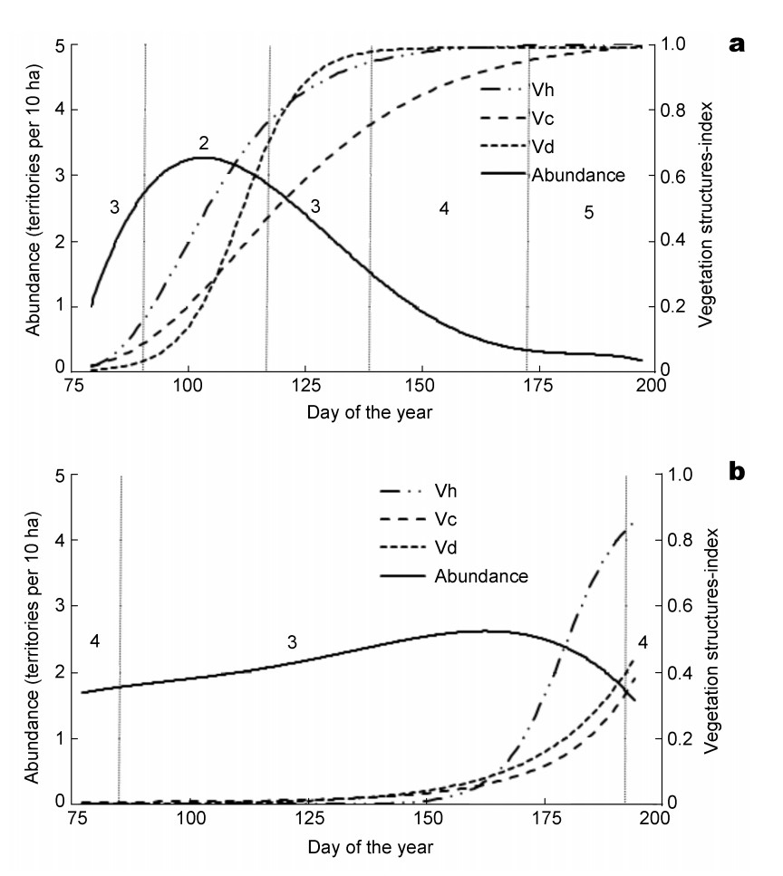
The comparison of abundances over the course of time with vegetation development leads to the assignment of abundance classes to vegetation height, coverage and density. The temporal variability of habitat suitability is thus related to the growth and development of the crops (Fig. 6). In winter rape, Skylarks find favorable habitat conditions (abundance class 2) for only a few days in mid-April. However, because a complete brood takes about 30 to 45 days (Bauer et al. 2005), the high abundances in this short time window cannot indicate the number of territories (approximately 2 or less per 10 ha). A second brood, obligatory for this species, will then be possible only for a fraction of the birds (less than about 20% of the individuals from the first breeding period).

Figure  6.  Dynamic abundance of Skylarks in winter rape (a) and maize fields (b) in relation to vegetation structure of the crops (Vh: height, Vc: coverage, Vd: density), habitat suitability classes: 2 – high, 3 – intermediate, 4 – low, 5 – very low.

DownLoad: Full-Size Img PowerPoint

In contrast to the pronounced temporal variability of Skylark habitat suitability in winter rape, the maize fields exhibited a more constant Skylark abundance on an intermediate (abundance class 3 and 4) level throughout the breeding season. In winter rape fields Skylark abundance reached a maximum on April 12, the maximum abundance in maize was nearly two months later on June 6, within the second breeding period. These contrasting abundance curves indicate a relationship exists between Skylark abundance and the development of vegetation structure, expressed as height, coverage and density in Fig. 6. In both crops Skylark abundance maxima occurred when the vegetation was thin and sparse.

Habitatmatrix (HM) of the Whinchat

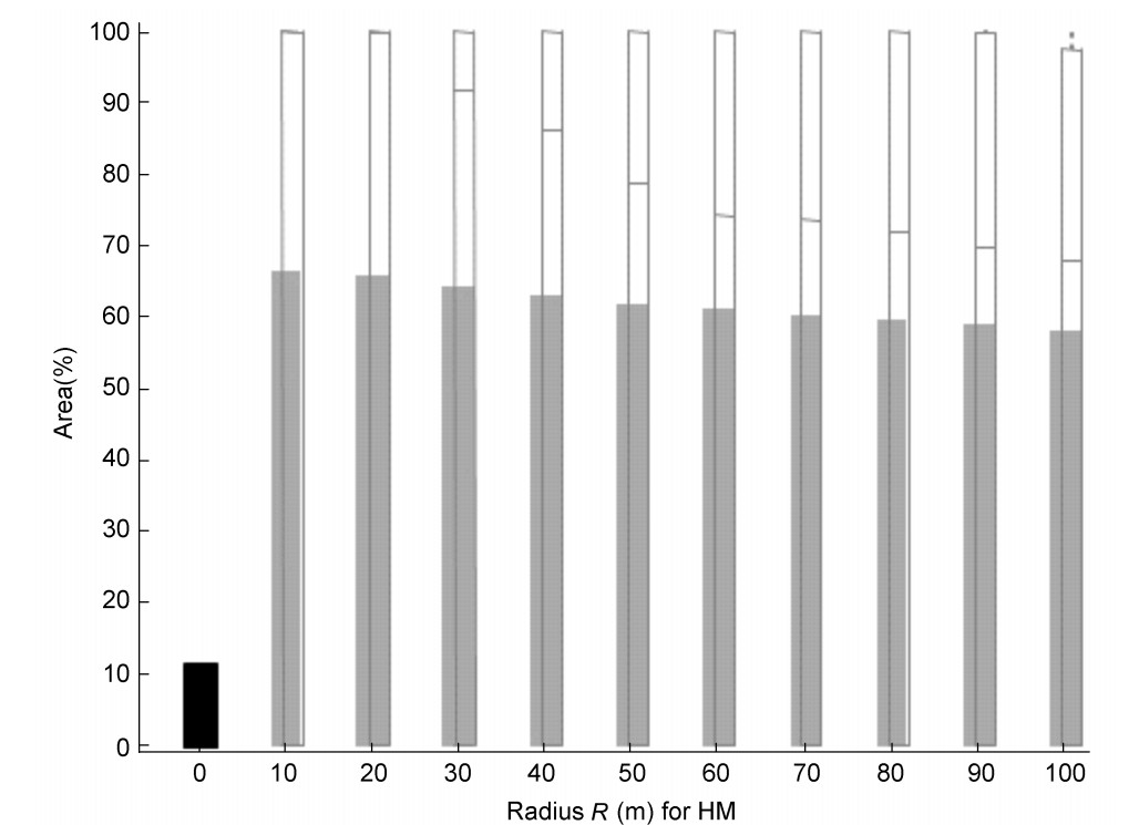
The Whinchat is a migratory bird species, typical for European open countryside areas with a preference for grasslands (Bauer et al., 2005). The first individuals were detectable in the study areas in the second half of April and then continuously to July (Table 5). During the breeding season a total of 193 TPs were located. The habitat matrix analysis was based on the spatial habitat composition of each HM in each survey to characterize the typical breeding habitat and possible changes to this habitat within the breeding season. The circular areas surrounding each TP (with r = 10 to r = 100 m), were analyzed, hence a total of 1930 Whinchat HMs. Table 8 shows the result of HM analysis for one survey (first half of June) as an example. The proportion of fallow land within the HMs decreased with increasing HM area, from 66% in the HM of 10m radius, to 57% with 100 m radius, and was significantly higher than the proportion within the entire landscape ('R₀'), which was 11.7% (Fig. 7).

Table  8.  Habitat Matrix (HM) of Whinchat territories (r = 70 m) in the course of time for the land use type 'fallow land'. TP – number of territory points, FLAL – fallow land area in the agricultural landscape (%), ATPEL – fallow land (average area in %) in all HMs (n = 193); TPFL – TP (number) with fallow land within HM, MA – mean area of fallow land (%), M – median (%), Q₁ – quantile 25%, Q₂ – quantile 75% for fallow land.

Time	TP	FLAL	ATPFL	TPFL	Statistical measures of HMs with fallow land
					MA	M	Q1	Q2
March 2	0	12.4	/	/	/	/	/	/
April 1	0	12.4	/	/	/	/	/	/
April 2	7	11.7	41.9	3	97.9	100	93.6	100
May 1	36	11.7	35.1	15	84.2	93.7	73.8	100
May 2	50	11.7	45.4	25	90.8	100	85.4	100
June 1	48	11.7	60.1	34	84.9	97.1	66.2	100
June 2	36	11.7	62.8	25	90.4	99.8	82.2	100
July 1	16	11.7	51.6	9	91.8	100	100	100

 | Show Table

DownLoad: CSV

Figure  7.  Proportion of the area covered by fallow land within the agricultural landscape (R₀ left on the x-axes) and within the 'Habitat Matrix' (HM) of the Whinchat from r = 10 m to r = 100 m (n = 48 territory points for survey 6, first half of June).

DownLoad: Full-Size Img PowerPoint

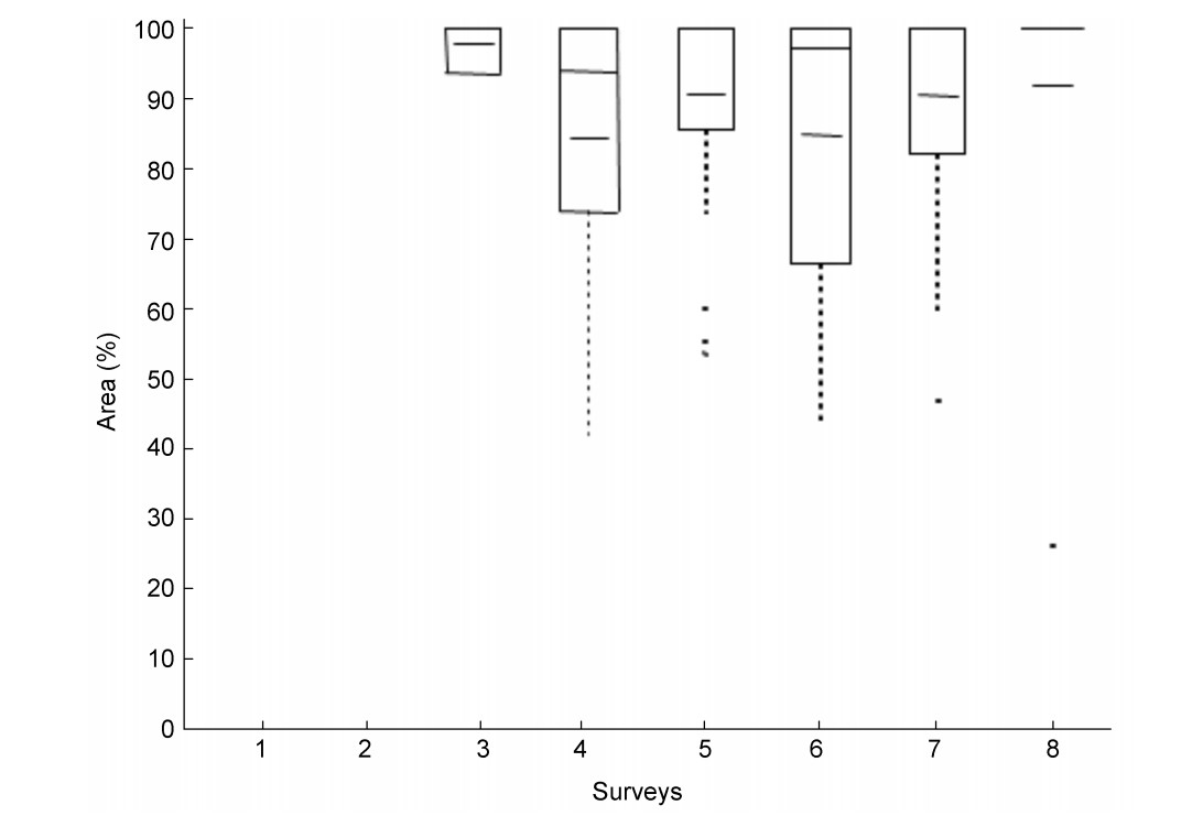
According to these results the Whinchat appears to select breeding habitats with a very high proportion of fallow land (similar to natural grassland) in the immediate surroundings of the TPs. In order to see if this preference is changing over the course of the breeding season, a comparison was made of the HMs with r = 70 m (1.54 ha) of the eight surveys. We chose r = 70 m since, according to Bauer et al. (2005), territories of Whinchat in Central Europe have an average area size of about 1.5 ha, varying from 0.5 to 3.5 ha. For each HM, the proportions of crops and habitat types (both in ha and percent) were quantified. Table 8 summarizes the relationship between all territories and the proportion of fallow land over the course of the breeding season. Whereas the total agricultural landscape was covered by fallow land by only 11.7% to 12.4 %, the Whinchat territories (r = 70 m) harbored significantly more, i.e. between 35% to 63% fallow land (Table 8). However, not all of the territories included fallow areas ('ATPEL' and 'TPFL' in Table 8). In those territories which contained fallow land (TPFL) the proportion of fallow was between 84% and 98% (Table 8 and Fig. 8).

Figure  8.  Proportion of fallow land in the Whinchat territories during the breeding time; (Habitat Matrix r = 70 m; fallow land > 0%; quantile 25%, quantile 75%, median mean), surveys from March (1) to July (8), n = 111 TPs, 2010.

DownLoad: Full-Size Img PowerPoint

All other land use types and habitats within the HM were quantified as described in the above example and related to the average proportion of that land cover type within the scale of the entire agricultural landscape (Table 9). In contrast to fallow land, both, maize and winter wheat fields were avoided by Whinchats during the breeding season. Maize and winter wheat cover 25% and 21% of the agricultural landscape, whereas only approximately 1.4% to 4.5% maize and 0.2% to 10.1% winter wheat were found in the HMs. From the beginning of the breeding season in April until the main breeding season in June, the proportion of fallow land increased successively from about 35% to 63% within the HMs, indicating essential habitat functions, whereas the coverage with winter wheat decreased from 10% to 0.2%. Similar to fallow land, seminatural grassland is also readily used by Whinchats. Although only 1.1% of the agricultural landscape was covered by this habitat type, within the Whinchat HMs the proportion of grassland was between 6 and 22 %. Next to fallow land, the habitat suitability of seminatural grassland was also high.

Table  9.  Comparison of the data with the proportion of the agricultural landscape and the territories of Whinchat (HM: Habitat Matrix, r = 70 m), both with the occurring land use types and habitats

Area of different land use type (%)
Fallow land			Winter wheat			Winter rape			Maize			Triticale			Other crops
Landscape	HM r 70		Landscape	HM r 70		Landscape	HM r 70		Landscape	HM r 70		Landscape	HM r 70		Landscape	HM r 70
12.0	35.1–62.8		21.0	0.2–10.1		24.0	3.6–15.8		25.0	1.4–4.5		3.3	0–5.0		9.8	8.4–21.7
Area of different habitat (%)
Hedges, small woodlands			Forest			Water bodies			Grassland			Urban areas			Traffic areas
Landscape	HM r 70		Landscape	HM r 70		Landscape	HM r 70		Landscape	HM r 70		Landscape	HM r 70		Landscape	HM r 70
1.1	1.4–2.1		0.6	0–0.9		1.0	0.6–2.3		1.1	6.0–22.4		0.5	0.3–0.6		0.2	0.3–0.6

 | Show Table

DownLoad: CSV

Table 9 summarizes the proportions of the crops and habitat types for the agricultural landscape, contrasted by the Whinchat HMs throughout the breeding season. This indicates the habitat preferences for the selection of breeding areas.

Discussion

Since its introduction the farmland bird indicator for biodiversity assessment used in Europe has displayed a negative trend. The indicator suggests an overall population decline of 52% since 1980 with an estimated loss of more than 300 million farmland birds over the last three decades (BirdLife International, 2012). This decline is closely related to changes in the agricultural landscape and the intensification of agricultural practices. Specifically, agricultural intensification has led to significant alterations on various scales, e.g., increased yields, related to more dense and homogeneous crop field vegetation on the scale of individual fields and decreased crop diversity on the landscape scale. In turn, this leads to more simple crop rotations, decreases in the proportion of seminatural habitats and results in food shortages for farmland birds. In particular, a long term increase in the use of pesticides has resulted in a decrease in food availability (e.g. Chamberlain et al., 2000; Newton, 2004; Flade et al., 2004; Donald et al., 2006; Wilson et al., 2009). Changes in land use are often dramatic and can occur rapidly. For example, in 2007 the EU regulation for set-aside (fallow land) promotion of approximately 10% of the agricultural area was abandoned. At the same time, the cultivation of socalled 'energy crops' was fostered. These two political decisions have led to profound changes in cropping patterns such as a rapid increase in maize production with a concomitant decrease in set-aside (for Germany see Flade et al., 2011) and impacts on crop rotations and crop diversity. Unfortunately, a further decrease of biological diversity in agricultural landscapes can be expected on regional, national and European levels. These decreases are in contrast to the aims of the sustainability strategy of the federal German government (BMU, 2007) and the EU biodiversity goals (COM, 2011).

Birds are often used as indicators for the evaluation of biodiversity (e.g. Morrison, 1986; EEA, 2007; Hoffmann and Kiesel, 2009; Sudfeldt et al. 2010; EEA, 2010), and farmland bird population changes should specifically be examined, analyzed and evaluated in relation to agricultural land use conditions and changes. The success of efforts to halt biodiversity decline is undoubtedly related to the understanding of cause-effect relationships. For the protection of farmland birds this is difficult in some cases, because most current farmland bird monitoring programs are based on point counts or line mapping, leading to incomplete coverage of the study areas (usually 1 km²). Small study areas such as these combined with incomplete coverage of the monitoring surveys make it difficult to determine the preferred habitats of breeding birds. Additional difficulties are due to the fact that important habitat characteristics for birds, like habitat coverage and vegetation structures are often not monitored. By the use of the territory mapping method with integrated habitat surveys, a better understanding of cause-effects relationships between landscape, land use features and farmland bird abundances is possible. In addition, the hierarchical structured monitoring scheme described in the current study allowed evaluations to be made on different spatial scales through 'zooming in' from the landscape level down to the single habitat and the breeding territory selected by individual birds, called 'Habitat matrix' (HM).

While large areas with less human impact than in agricultural areas (national parks, biosphere reserves, nature conservation areas etc.) are most important for the protection of biological diversity, agricultural areas have significant importance for farmland birds and bird species diversity both in general and worldwide (Weijden et al., 2010). In this study, 50% of all breeding bird species in the Federal State of Brandenburg (approx. 30000 km²) were detected within a 29 km² sample of 'typical, common' agricultural landscape. This indicates the high potential value of the rural areas for nature conservation. Agricultural landscapes can support biodiversity but the extent of this support is dependent on the intensity of agricultural practice, the proportion of seminatural habitats (Hoffmann et al., 2000, 2012), and the spatial land use structure. Well-documented declines in the populations of many European farmland bird species (e.g. Donald et al., 2001; BirdLife International, 2004; Sudfeldt et al., 2010; Flade et al., 2011; EBCC, 2012) suggest that the conservation measures employed to stop these negative trends are not adequate. Hence, the biodiversity function of agricultural landscapes is at stake if land use intensification continues without the simultaneous implementation of more effective bird protection measures.

In order to achieve this, the identification of the habitat requirements of selected indicator farmland bird species, for Germany and Europe for example Corn Bunting, Skylark and Whinchat (Achtziger et al., 2004, EEA, 2007) can be useful. The case of the Corn Bunting reveals large differences in breeding bird abundances on various spatial scales, depending on the landscape structures and the type of management on the agricultural fields, especially crop vegetation characteristics.

As the example of the Skylark demonstrates, it is important for the description of abundance as a dynamic function for the whole breeding season to select meaningful variables for the cropping patterns on the landscape scale and for crop vegetation structures for the habitat quality. As observed by Schön (2011) in this case, the identification of the dynamic abundances within different breeding habitats helps to detect habitat qualities and favourable vegetation structures in crop fields and habitats. Using this methodology for specific crops, it should be possible to identify those time windows within the growing period which are best suited to meet the breeding requirements of individual farmland bird species. However, more research is needed to test the relation between the territory mapping method, which is based on observations on bird behavior, and the true abundances. This is due to the fact that some of the species behavioral activities depend on the season and underestimation of abundances is possible when a specific behavior is not displayed. This information can be useful for crop management schemes aimed at protecting and supporting specific farmland bird species and can be applied to both individual crops and the spatial arrangement of land use types (see Morris et al., 2004; Wilson et al., 2005; Fischer et al., 2009).

HM-analysis demonstrated here using the example of the Whinchat, allows the identification of the preferred field crops and other habitats and their spatial proportions by the breeding bird species. HM-analysis can therefore help to identify potential causes of changes in farmland bird populations as a result of changes in agricultural cropping patterns and land use and in doing so, provide a basis for bird protection strategies within changing agricultural landscapes.

However, any strategy or action aimed at countering the loss of farmland bird diversity and abundance will require reliable and quantifiable parameters for bird occurrence and their use of the landscape. We suggest that the bird population data sets (species diversity, dynamic abundances, STDA, HM) used here combined with the hierarchical approach on land use (agricultural landscape, agriculture landscape types, field crops and other habitats, vegetation structures) may be suited to serve this purpose. In particular an adequate number of monitoring surveys (eight) conducted from the beginning to the end of the breeding season combined with measurements and assessments of the crop vegetation and vegetation structural development, for the interpretation of these data helps to understand why bird species will or will not occur and breed in specific agricultural areas. While simple abundance data may reveal relations between bird species and the general agricultural landscapes, specific field crops or habitat types in agricultural landscapes, such data can neither be related to the spatial arrangement of habitats nor to vegetation structures within the bird breeding territory. Consequently, we suggest that the HM concept can fill this gap as it provides information on the actual habitat preferences of farmland birds on various temporal and spatial scales. Furthermore, HM-analysis helps to forecast changes in farmland bird population by proposing cause-effect relationships between these populations and changes to cropping schemes, habitat distributions and vegetation structures. In order to reach the goals of globally promoted biodiversity conservation and enhancement (COM, 2011), it is important that agricultural practices incorporate the principles of biodiversity conservation because arable fields are habitat to many species. Methods such as abundance monitoring, STDA, characterisation of vegetation structures and HM-analysis, particularly when used in combination, have the potential to provide reliable predictions on habitat suitability for farmland birds in changing landscapes. In order to be effective, the design of measures aimed at supporting biodiversity, e.g. agri-environmental schemes (AES), require better knowledge of the habitat requirements of indicator species. Accordingly, methods such as these can be used to support measures to save and enhance biodiversity within agricultural landscapes. Some EU AES programs are specifically intended to enhance biodiversity. However, the well-documented continued decline of biodiversity in rural landscapes clearly shows a discrepancy between political goals and the efficacy of the current AES program. To enhance the efficiency of AES and nature conservation efforts in general, it seems helpful to identify those agricultural practices, habitat types and spatial habitat compositions with high habitat quality values for indicator species and thus for biodiversity in general. We suggest applying national monitoring programs with a hierarchical structured spatial design in which bird species abundances can be related to important characteristics of the agricultural landscape for efficient biodiversity conservation. Accordingly, we recommend that biodiversity data and data on land use should be gathered simultaneously and on the same areas.

Acknowledgements

Funding from the German Federal Ministry of Food, Agriculture and Consumer Protection (BMELV). Many thanks to Jan-Dieter Ludwigs for useful information and Andy Ranstall for improving the English and valuable comments.