Xhareni Díaz-Lezama, Alejandro Ariel Ríos-Chelén, Jorge Castellanos-Albores, Paula L. Enríquez. 2025: Are urbanization, biotic and social factors associated with the song frequency and song entropy attributes of three urban syntopic passerines?. Avian Research, 16(1): 100219. DOI: 10.1016/j.avrs.2024.100219
Citation:
Xhareni Díaz-Lezama, Alejandro Ariel Ríos-Chelén, Jorge Castellanos-Albores, Paula L. Enríquez. 2025: Are urbanization, biotic and social factors associated with the song frequency and song entropy attributes of three urban syntopic passerines?. Avian Research, 16(1): 100219. DOI: 10.1016/j.avrs.2024.100219
Xhareni Díaz-Lezama, Alejandro Ariel Ríos-Chelén, Jorge Castellanos-Albores, Paula L. Enríquez. 2025: Are urbanization, biotic and social factors associated with the song frequency and song entropy attributes of three urban syntopic passerines?. Avian Research, 16(1): 100219. DOI: 10.1016/j.avrs.2024.100219
Citation:
Xhareni Díaz-Lezama, Alejandro Ariel Ríos-Chelén, Jorge Castellanos-Albores, Paula L. Enríquez. 2025: Are urbanization, biotic and social factors associated with the song frequency and song entropy attributes of three urban syntopic passerines?. Avian Research, 16(1): 100219. DOI: 10.1016/j.avrs.2024.100219
Programa de Posgrado en Ciencias en Recursos Naturales y Desarrollo Rural, El Colegio de la Frontera Sur. Carr. Panamericana y Periférico Sur s/n Barrio Ma. Auxiliadora, 29290. San Cristóbal de Las Casas, Chiapas, Mexico
b.
Centro Tlaxcala de Biología de la Conducta, Universidad Autónoma de Tlaxcala, Universidad 1, La Loma Xicohtencatl, Centro, 90000, Tlaxcala, Mexico
c.
Departamento Conservación de la Biodiversidad, El Colegio de la Frontera Sur, Carr. Panamericana y Periférico Sur s/n Barrio Ma. Auxiliadora, 29290 San Cristóbal de Las Casas, Chiapas, Mexico
Funds: We thank the Consejo Nacional de Humanidades, Ciencias y Tecnologías (CONAHCYT) of Mexico for providing funding for graduate studies of X.D.L. (No. 001283). We are also grateful to El Colegio de la Frontera Sur for PATM graduate fellowship for fieldwork
Urban environments have challenging characteristics for bird acoustic communication. High levels of anthropogenic noise, as well as vegetation structure (e.g., in urban parks), can potentially affect the song frequency characteristics of several bird species. An additional factor such as the abundance of conspecific and heterospecific vocalizing birds may play an important role in determining the structure of bird songs. In this study, we analyzed whether noise levels, vegetation percentage, and abundance of conspecifics and heterospecifics influence the song characteristics of three syntopic songbird species: House Finch (Haemorhous mexicanus), Rufous-collared Sparrow (Zonotrichia capensis), and House Sparrow (Passer domesticus) living in urban sites. We recorded songs of these species and measured the peak frequency and entropy of their songs at 14 sites in the city of San Cristobal de Las Casas, Chiapas, Mexico. We found that the song peak frequency of House Finch and House Sparrow’s songs was negatively related to the vegetation. The peak frequency of neither of the three species correlated with the average noise level. However, the abundances of conspecific and heterospecific were related to the peak frequency of the three species’ songs. The entropy of the House Finch and House Sparrow songs was positively and negatively related, respectively, to noise levels. House Sparrow song entropy was negatively related to the percentage of vegetation. Song entropy of House Finches was negatively associated to conspecific and House Sparrow abundance. Song entropy of Rufous-collared Sparrows was positively related to conspecific abundance. In conclusion, the song peak frequency and song entropy of the three songbird species were differentially related to urban noise, vegetation, and conspecific and heterospecific abundance, suggesting these factors influence bird song characteristics.
Urban sites have very different acoustic characteristics from natural environments, which can be a challenge for the effective transmission of the songs of birds living in cities. In general, cities share common characteristics such as high levels of anthropogenic noise, the presence of large reflective surfaces (vertical buildings), as well as fragmented and sparse vegetation (Brumm, 2004; Hu and Cardoso, 2009; Dorado-Correa et al., 2016). These urban characteristics represent unfavorable conditions for sound transmission, potentially degrading the original structure of bird songs and altering the message they transmit. However, some bird species have been able to successfully colonize urban habitats; to achieve this, they have undergone behavioral changes for mating and breeding in specific sites such as houses and buildings, diversifying behavior and even modifying their songs and vocal behavior (Ey and Fischer, 2009; Nemeth and Brumm, 2009; Winandy et al., 2021).
Several song acoustic characteristics, including amplitude, frequency (pitch), and song structure, determine the propagation of a signal through an environment (Barker, 2008; Nemeth and Brumm, 2010; Mikula et al., 2021). When it comes to anthropogenic noise, its energy is generally concentrated in low frequencies (below 3 kHz); therefore, vocal signals with low frequencies can be easily masked (Hu and Cardoso, 2009). Faced with anthropogenic noise, several species increase the signal-to-noise ratio (Slabbekoorn et al., 2007; Nemeth and Brumm, 2009; Mendes et al., 2011); that is, the proportion of signal energy to noise energy, where higher values result in an increased probability of signal detection. One strategy that results in a higher signal-to-noise ratio, is to increase the frequency of vocal sounds, which can improve signal transmission (e.g., Nemeth and Brumm, 2010; Laiolo, 2011). At the same time, some bird species decrease the frequency or frequency bandwidth of their vocalizations in noisy environments, resulting in an increased transmission and tonality (Hanna et al., 2011; Potvin et al., 2014).
Increasing the tonality of the signals represents an alternative strategy to increase the signal-to-noise ratio. Pure tone signals have narrow bandwidth that transmit better through noisy habitats than signals with higher bandwidth (Lohr et al., 2003; Hanna et al., 2011). Song entropy can give information on how tonal a song is, and it is defined as the randomness of a sound; pure tones will have an entropy value close to 0, while white noise will have an entropy value close to 1 (Hanna et al., 2011). Some species may increase the tonality of their songs when exposed to low-frequency noise (Hanna et al., 2011). The Eurasian Wren (Trogloytes troglodytes) emit songs with lower entropy in noisier urban sites than in less noisy rural sites (Colino-Rabanal et al., 2016).
Urban sites are also environments with vertical building structures and a different vegetation composition than natural sites, so birds face heterogeneous habitats with different acoustic properties than natural environments. Both vegetation structure (Azar and Bell, 2016) and building materials in urban areas can influence how birds vocalize (Job et al., 2016). The Acoustic Adaptation Hypothesis establishes that habitat structure and its acoustic properties influence sound transmission, shaping the evolution of acoustic signals; therefore, several fauna species such as birds will adjust their vocal signals to decrease degradation in the environment (Morton, 1975; Hansen, 1979; Ey and Fischer, 2009). Sounds are more degraded and attenuated in closed environments than in open spaces, and it is sounds with lower frequencies and with a narrower bandwidth (with less entropy, more tonal) that are better transmitted in closed environments (Konishi, 1970; Morton, 1975; Boncoraglio and Saino, 2007). On the other hand, in open sites higher frequency sounds and frequency-modulated acoustic signals are better transmitted (Morton, 1975). Construction and building materials in urban areas can also influence bird vocalizations (Slabbekoorn et al., 2007; Job et al., 2016); some birds decrease peak frequency as urban structure increases, which may help to decrease the accumulation of reverberations produced by buildings (Slabbekoorn et al., 2007; Job et al., 2016).
Birds vocalizing in urban sites face, in addition to urban noise and vertical constructions, sounds emitted by other bird species (Doutrelant et al., 2000; Azar and Bell, 2016). Communities of birds in urban areas will likely be determined to some extent by a homogenization process (Groffman et al., 2014), where, for instance, some non-native species thrive at the expense of other native species (McKinney, 2006). If bird species in these communities have similar frequency characteristics, as well as similar times and spaces to vocalize, then they occupy the same acoustic niches (Kennedy et al., 2023), increasing the possibility of song overlap. Density of individuals is another factor that can encourage the modification of song parameters, because a high density will imply more intense and frequent social acoustic interactions (Nemeth and Brumm, 2009). To avoid this acoustic interference birds may undergo acoustic space partitioning, which is a multidimensional space composed of features such as peak frequency, duration, number of notes and other features of song structure (Kirschel et al., 2009; Luther and Wiley, 2009).
According to the Acoustic Niche Hypothesis, species have their own acoustic niches with unique temporal and frequency characteristics, where they avoid frequency and temporal overlap with signals from other vocal individuals in their environment (Krause, 1993). Birds in the same community are then expected to decrease similarities in frequency characteristics to avoid song overlap and competition for acoustic space (Azar and Bell, 2016). Alternatively, regardless of song frequencies, birds may use different timings to sing, avoiding temporal overlap. In allopatry, closely related species tend to have similar songs (Haavie et al., 2004; Luther, 2009); however, in sympatry their songs will differ spatially and temporally (Kirschel et al., 2009; Cardoso and Price, 2010). Some bird species decrease the peak frequency of their songs and others increase it depending on which species they are in sympatry with (Kirschel et al., 2009). For instance, Rumped Tinkerbirds (Pogoniulus bilineatus) and Yellow-throated Tinkerbirds (P. subsulphureus) decrease and increase, respectively, song peak frequency when in sympatry (Kirschel et al., 2009). Recent studies found that social factors (mate fertile status and number of neighbors), time of the day and season, but not noise levels, are associated with song frequency parameters of House Wrens (Troglodytes aedon) and Leaf Warblers (Grabarczyk et al., 2020; Deoniziak and Osiejuk, 2021).
In cities, all these factors (noise, vegetation, vertical structures and abundance of sympatric vocal species) can act as selective pressures and shape bird song attributes. Three species that have apparently adapted well to urban conditions are the House Finch (Haemorhous mexicanus), the Rufous-collared Sparrow (Zonotrichia capensis), and the House Sparrow (Passer domesticus). These songbirds live in syntopy (i.e., "species using the same habitat"; Hart et al., 2018) in the city of San Cristobal de Las Casas, state of Chiapas, Mexico, and emit songs (Fig. 1). The House Finch is a native non-territorial and social bird with quite complex and long songs, with the ability to increase the minimum frequency of their songs in noisy conditions (Bermúdez-Cuamatzin et al., 2009, 2010). This species is gregarious and tolerant of conspecifics. Agonistic interactions are mainly during feeding, at roost sites or during breeding. Although in urban areas this species can nest in proximity making colonies (Badyaev et al., 2020). The Rufous-collared Sparrow is a resident and territorial bird with a wide distribution in the American continent. The song of this species is exclusive to males, which is solitary and forms pairs during the breeding season. It has been shown that males start the dawn chorus earlier in noisy environments than their counterparts in quieter areas (Dorado-Correa et al., 2016). Additionally, the Rufous-collared Sparrow shows song geographic variation and associations between song temporal and frequency attributes with habitat type (Hanford and Lougheed, 1991). On the other hand, the House Sparrow was introduced in North America with great success; therefore, it is common and gregarious all year long. It is a monogamous species, and the male shows a sexual display and a ritual for breeding generally in communal displays. Breeding occurs in small colonies (Lowther and Cink, 2020). House Sparrows do not defend a territory, but they defend a small area around the nest (McGillivray, 1980; Tobias et al., 2016). It shows great vocal activity throughout the day and is considered a pest species by some authors, potentially displacing native species (Murgui and Macías, 2010; Berigan et al., 2020). In addition, it has been described that these three species can compete for other resources such as nesting sites or food (Cadena-Ortiz, 2018; Menacho et al., 2018). If these three species share the same niche of acoustic space, then this may result in competition, which in turn could shape the characteristics of their songs.
Figure
1.
Song spectrograms of three passerine bird species: (A) House Finch, (B) Rufous-collared Sparrow, (C) House Sparrow. Recorded in San Cristóbal de Las Casas, Chiapas, February–April, 2021.
In this study, we evaluated whether and how noise level, the percentage of vegetation and conspecific and heterospecific abundance are associated with song characteristics of each of the three songbird species: the House Finch, the Rufous-collared Sparrow, and the House Sparrow. From the songs of the three species, we analyzed the peak frequency and entropy. We predicted that: 1) the song peak frequency of each species will be positively related to noise level (which may reduce noise overlapping with song frequencies); 2) song peak frequency of each species will be negatively related to the percentage of vegetation (concentrating more energy in lower frequencies may reduce the loss of song energy as it passes through the vegetation); 3) conspecific and heterospecific abundances will be related positively or negatively with the song peak frequency of the birds (diverging song frequency when there are many individuals of the same or different species may prevent song overlap); 4) song entropy will be negatively related to urban noise levels (less entropic songs have a higher probability of detection and transmission in noise); 5) song entropy will be positively related to the abundance of individuals (both conspecific and heterospecific), since more entropic songs may be perceived as more aggressive signals (Furutani et al., 2018) and may help males defend their territory and/or chicks in the nest; 6) song entropy will be negatively related with vegetation (sounds with less entropy are more tonal and have a narrower bandwidth, which enhances transmission in densely vegetated environments).
2.
Materials and methods
2.1
Study area
We conducted this study in 14 urban sites in the city of San Cristóbal de Las Casas (16.7317° N and 92.6375° W, 2121 m above sea level), Chiapas, Mexico (INEGI, 2017, Fig. 2). The climate in the city is temperate subhumid with summer rainfall, with mainly pine-oak forest vegetation (INEGI, 2017). The annual temperature in the city of San Cristóbal de Las Casas ranges from 12 to 24 ℃ and the annual precipitation ranges from 1000 to 1500 mm. The three species of passerines (House Finch, Rufous-collared Sparrow, and House Sparrow) were present in all 14 sampling sites, where they are exposed to different sources of anthropogenic noise (vehicular and noise from people). The sites were selected according to their reachability, trying to capture a wide variation in noise levels, and vegetation and construction percentage. The sites were surrounded by man-made buildings and harbored green areas or gardens. This meant that sites varied in size, as observations were limited by visual obstacles (e.g., walls). We recorded bird songs during the months of February, March, and April of 2021, during the period of highest vocal activity of the three species. We visited each site 13 times to capture the variation in song characteristics and noise levels. The average distance between the sampling points was 1926 ± 989 m (Fig. 2) and the geographic coordinates of each site were obtained with a Garmin GPS Navigator GPSMAP 64SX.
Figure
2.
Study area and fourteen sites where songs of the House Finch (Haemorhous mexicanus), Rufous-collared Sparrow (Zonotrichia capensis) and House Sparrow (Passer domesticus) were recorded from February to April 2021 at San Cristóbal de Las Casas, Chiapas state, Mexico.
Tall structures (shrubs, trees, houses) may affect more strongly the transmission of acoustic signals than flat surfaces. We classified landscape features into three categories: vegetation, human built structure, and flat surface. We determined the percentage of vegetation cover and construction with a supervised classification using ArcMap 10.8 software. For this analysis, a 2021 satellite image with a resolution of 10 m was used to characterize each point sampled in San Cristóbal. To determine the percentage coverage of green areas and human constructions, a supervised classification was performed in the ArcMap 10.8 program. For this analysis, a Sentinel 2 image of 2021 with a resolution of 10 m was used for the urban area of San Cristóbal, where the recording points were located. For the classification of the two coverage classes, training areas were established (sites where the presence of green areas which included trees and shrub-type vegetation), which allowed obtaining an image with these two coverage classes. Subsequently, a shapefile was generated with the polygons of the coverages. In the generated image, the recording points were overlapped to create buffers of 50 m radius (7850 m2). A 50 m buffer was selected because at some points the buffers overlapped. In the area of the buffers, the coverage of green areas and construction was estimated in square meters, and finally the percentage of these two classes in each point was calculated. We also considered a third category of flat surface, such as any surface that was made up of grass or cement cover.
2.3
Song recordings and sound analysis
At each site, the recordings were made with a SONY PCM-M10 digital hand-held recorder (sampling rate 44 kHz and 16-bit precision), connected to an Audio-technical AT8035 shotgun condenser microphone. Only the songs of males of each species were recorded. Male House Finches and House Sparrows were easy to distinguish visually due to the sexual dimorphism of their plumage. Rufous-collared Sparrows are not sexually dimorphic in morph, so we distinguished males from females because males were the ones actively singing at the time of recording, and females in this species rarely sing (King, 1972). Each recording period consisted of at least 1 min, except in cases where the bird flew away or stopped singing before the end of the recording period. The recording periods were from 06:30 to 11:00 a.m., avoiding recording days with rain and wind greater than 3 m/s (Mendes et al., 2017). At the start of the recordings, we pointed the unidirectional microphone toward the focal bird at 5–10 m. The greater tolerance of the House and Rufous-collared Sparrows to human proximity allowed us to record them at a distance as short as 1–2 m. When there was more than one male vocalizing at the same time, the microphone was directed towards the new individual only after obtaining a minimum of 5–10 songs from the previous male.
Each recording was numbered by species, and for the analysis 30 recordings per site and species with random numbers were selected. In total, we analyzed 1080 songs, 420 songs of Rufous-collared Sparrow, 420 of House Sparrow, and 240 songs of House Finch. We only analyzed 240 House Finch songs because in some sites we did not obtain the minimum number of songs of sufficient quality to analyze (as it did not vocalize enough). We only measured songs with sufficient quality (i.e., no background noise interference, no overlapping of other sounds). For each species 30 recordings were selected, and within each recording an individual song was selected to measure peak frequency and entropy. Subsequently, the average of peak frequency and entropy per site was obtained; these means were used in further analyses. We measured the peak frequency of the song (Hz) and the average entropy with Raven Pro1.6.3 (https://www.birds.cornell.edu/ccb/raven-pro/). As a measure of song pitch, we chose the peak frequency of the song because this is a robust parameter; this measurement is largely unaffected by the quality of the recording or background noise. Entropy is a measure of the amount of information contained in a signal and allows us to know how complex, and random a song is (Shannon and Weaver, 1964; Sandoval et al., 2018). Higher entropy values indicate more random and disordered sounds, while lower entropy sounds are more tonal (Hanna et al., 2011).
The songs selected were of good quality (duration and frequencies of all notes clearly marked on the spectrogram). Before measuring each song, we removed background noise with the "filter out active selection" function in Raven. With this function, all sounds below 1 kHz were removed, taking care that the focal song was intact. Each song was selected manually by clicking on the spectrogram and dragging the cursor so that the selection range surrounded the target song. The beginning and ending of each song were determined with the help of the waveform. After selecting the song, Raven automatically measured its peak frequency and average entropy.
2.4
Environmental noise
Noise levels were obtained with a digital sound level meter EXTECH 407730 (range 20–130 dB, Type 2 ANSI S1.4–1983, A weighting, fast response), and with a similar method used by Brumm (2004). Noise was measured by placing the sound level meter horizontally to the ground, and we always started measuring the noise pointing North and then measured the next cardinal points (East, South, and West) by moving the sound level meter clockwise. We obtained a single measure of minimal and maximum noise level in a period of 60 s, before turning the sound level meter to another cardinal direction. As we visited each site 13 times (see Section 2.5 Abundance below), we ended up with several noise recordings for each site. Noise levels were taken 10 min before we started recording the songs. The minimum and maximum noise values were averaged to obtain a mean noise value for each site; these means were used in further analyses. Noise measures are reported in dB SPL re 20 μPa.
2.5
Abundance
To estimate the relative abundance of the species at each sampling site, we used the point count method. As observations were limited by visual obstacles in the environment (e.g., buildings), we used the point count method without a fixed radius. This method consisted of counting all individuals per species, during a period of 10 min. The observer (X.D.L.) used 10–30 × 50 Celestron-Prismatic binoculars, and the average maximum radius from the count points was no more than 30 m. Point counts are a simple and versatile method that can be used in different environments (Hutto and Stutzman, 2009). Abundance estimations and ambient noise measures were taken at the same time and day as the song recordings. Each sampling point was visited on 13 different days to estimate the abundance (number of individuals per count point).
2.6
Statistical analysis
Nonparametric tests (Kruskal–Wallis) were used to determine differences in noise levels, vegetation percentage, species abundances, song peak frequencies and song entropy among sites, and song peak frequencies and song entropy between species. Initially, we performed exploratory correlation analyses to define whether there were correlated variables. These analyses revealed that the percentage of vegetation and the percentage of construction were highly correlated (Spearman correlation: r = −0.819, p < 0.001). The percentage of flat area was also correlated with the construction (Spearman correlation: r = −0.853, p < 0.001). In addition, flat surface was not a consistent variable in all sites (it was present only in six out of 14); therefore, we only used the percentage of vegetation in further analysis. We ran Generalized Linear Models (GLMs), with normal distribution and identity link, to analyze the relationships between song acoustic variables of each songbird species and average noise levels, percentage of vegetation, and abundance of focal species. Because we did not mark birds and recorded more than one bird per site, the chances of recording an individual more than once per site were high. Therefore, and to avoid pseudoreplication, we averaged the data per site and used these means in further analyses. Thus, to run the GLMs, we used a database with site means for each acoustic parameter (song peak frequency and song entropy) for each species. Several models were constructed, and the Akaike Information Criterion (AIC) values were compared to choose the best model. In GLMs, the models with the lowest AIC value are those with the best fit, and a significant difference between models is considered to exist if there is a difference equal to or greater than two between AIC values. The first model built for each species included all the explanatory variables measured (percentage of vegetation, average noise level, conspecific abundance, and the abundance of heterospecific). In the following models, variables that had no significant effect were discarded until the model showed only variables significantly related to the acoustic parameters of each bird species. We corrected the P-values with Bonferroni. To do so, we divided the obtained P-value for each predictor variable in each model by the total number of predictor variables in each model. Only P-values from best models (those with lowest AIC value and with an AIC value difference of less than 2), that were used to interpret the results, were corrected. All statistical analyses were performed with SPSS 28.0 software (IBM Corp., 2021).
3.
Results
3.1
Exploratory analyses: noise, vegetation, and species abundance
In most sites, the principal source of noise was vehicular traffic, and in other sites it was due to anthropogenic activities (i.e., work machinery, pedestrians and people working). The minimum and maximum levels of noise varied significantly between sites (minimum noise, H13 = 85.20, p < 0.001; maximum noise, H13 = 76.99, p < 0.001). Minimum noise levels ranged from sites with 44.95 ± 2.37 dB (mean ± SE) to sites with 53.3 ± 2.22 dB, while maximum noise levels were between 56.34 ± 1.52 dB and 81.48 ± 4.30 dB. The average noise level also varied between sites (H13 = 95.01, p < 0.001; Fig. 3A) and ranged between 50.42 dB ± 1.68, and 66.24 dB ± 12.43. The percentage of vegetation varied from 0 to 50% between sites (Table 1). The noisier sites were less dense in vegetation (average noise level versus vegetation percentage, Spearman rho, r = −0.638, p = 0.014, n = 14).
Figure
3.
Site, noise levels, and abundance of three songbird species. (A) sites differed in noise levels. (B) abundances of the three songbird species (House Sparrow, House Finch, and Rufous-collared Sparrow) differed among sites. For explanations of site names, refer to Table 1.
Table
1.
Percentage of vegetation cover, construction cover, and flat surface in San Cristóbal de Las Casas, Chiapas, México.
No.
Site
% Vegetation
% Construction
% Flat surface
7
A Gpe
0
100
0
1
PN
0.50
81.66
17.83
5
I Sn Fco
1.01
98.98
0
11
UA
2.54
97.45
0
14
P Ma Aux
2.54
97.45
0
13
Alba 1
3.82
28.96
67.21
10
I Gpe
4.07
95.92
0
6
HM
11.96
88.03
0
9
Na Bolom
16.91
83.08
0
2
T de Cd
24.19
47.11
28.69
8
CC
28.01
71.98
0
3
SEDEM 2
41.71
24.83
33.50
4
SEDEM 1
42.35
8.91
48.74
12
Alba 2
50.36
13.37
36.27
Percentage of vegetation (% vegetation), any green surface with plants other than short grass (e.g., shrubs, trees); percentage of construction (% construction), any non-flat and man-built area (e.g., houses, buildings); percentage of flat surface (% flat surface), any flat surface (i.e., short grass or cement floor). Data are organized from lowest to highest vegetation cover. Numbers refer to study site numbers shown in Fig. 2. A Gpe, Andador Guadalupe; PN, Panteón; I Sn Fco, Iglesia de San Francisco; UA, Unidad Administrativa; P Ma Aux, Parroquia María Auxiliadora; Alba 1, Albarrada 1; I Gpe , Iglesia de Guadalupe; HM, Hospital de la Mujer; T de Cd, Teatro de la Ciudad; CC, Casa de la Cultura.
The abundances of the three species also differed between sites (House Finch H13 = 92.07, p < 0.001; Rufous-collared Sparrow H13 = 55.83, p < 0.001; and House Sparrow H13 = 85.04, p < 0.001; Fig. 3B). The abundances of House Finch and House Sparrow were not related to the percentage of the vegetation (Spearman rho, n = 14; House Finch, r = 0.152, p = 0.604; House Sparrow, r = −0.396, p = 0.161). However, the abundance of Rufous-collared Sparrows increased as the percentage of vegetation increased (Spearman rho, r = 0.590, p = 0.026, n = 14). The abundance of House Finches and Rufous-collared Sparrows was not associated with average noise levels (n = 14; House Finch, Spearman rho, r = −0.455, p = 0.102; Rufous-collared Sparrows, Pearson’s correlation, r = −0.49, p = 0.071); House Sparrows were more abundant in quieter areas (Pearson’s correlation, r = 0.63, p = 0.015, n = 14).
Estimated abundances differed between species (H2 = 13.39, p = 0.001). The abundance of House Finches (mean ± SE, 2.6 ± 0.8 individuals per site, range 0–10.6) was lower than that of House Sparrows (mean ± SE, 8.0 ± 1.1 individuals per site, range 1.3–15) (Dunnett test, p = 0.002) and only marginally and non-significantly lower than that of Rufous-collared Sparrows (mean ± SE = 4.8 ± 0.6 individuals per site, range 0.2–9.5) (Dunnett test, p = 0.068). The abundance of House Sparrows did not differ from that of Rufous-collared Sparrows (Dunnett test, p = 0.121).
3.2
Acoustic variables of the songs
Song peak frequency differed between species (H2 = 21.83, p < 0.001). The peak frequency of the song (mean ± SE) of House Finches (3604 ± 31 Hz, range 3476–3758 Hz, n = 8) was lower than that of House Sparrows (4135 ± 104 Hz, range 3594–4964 Hz, n = 14) (Dunnett test, p = 0.001) and Rufous-collared Sparrows (4503 ± 43 Hz, range 4266–4760 Hz, n = 14) (Dunnett test, p < 0.001). House Sparrows sang with a lower peak frequency than Rufous-collared Sparrows (Dunnett test, p = 0.013).
Song entropy also varied between species (H2 = 25.37, p < 0.001). Song entropy (mean ± SE) did not differ between the House Finch (3.37 ± 0.07, range 3.09–3.69, n = 8) and the House Sparrow (3.23 ± 0.03, range 3.01–3.51, n = 14) (Dunnett test, p = 0.332), However, Rufous-collared Sparrows (2.54 ± 0.03, range 2.27–2.87, n = 14) sang with a lower entropy than the other two species (p < 0.001).
3.3
Acoustic variables, noise level, vegetation, and species abundance
For House Finch (Table 2, models 1 and 2; Fig. 4A) and House Sparrow (Table 3, model 1–3; Fig. 5A) we found a negative relationship between their song peak frequency and the percentage of vegetation. The peak frequency of House Finch’s song was negatively related to the abundance of its conspecifics and to the abundance of its heterospecific House Sparrow (Table 2, models 1 and 2; Fig. 4B–D). However, its song peak frequency was positively related to the abundance of Rufous-collared Sparrow (Table 2, models 1 and 2; Fig. 4C). For the House Sparrow, we found that its song peak frequency was positively related to the abundance of House Finches and the abundance of its conspecifics (Table 3, models 1–3; Fig. 5B). For Rufous-collared Sparrow, there was no significant relationship between its song peak frequency and any of the measured variables (Table 4, models 1 and 2). We found no association between average noise levels and song peak frequency, this was true for the three studied species (Tables 2–4).
Table
2.
Comparison of different GLM (Generalized Linear Models) of peak frequency of the House Finch song in San Cristóbal de Las Casas, Chiapas, México.
Explanatory variables: percentage of vegetation, average noise, conspecific abundance, Rufous-collared Sparrow abundance and House Sparrow abundance. Models were ordered from best (model 1) to worst (model 5) according to their AIC values, and only the first two models were used to interpret the results (see text for details). P values were Bonferroni adjusted for these models only. Model 1 p ≤ 0.012, model 2 p ≤ 0.01. Significant values in bold.
Figure
4.
Peak frequency of House Finch songs, vegetation percentage, and conspecific and heterospecific abundance. (A) Peak frequency of House Finch songs decreased with vegetation percentage, (B) decreased with conspecific abundance, (C) increased with Rufous-collared Sparrow abundance, and (D) decreased with House Sparrow abundance.
Table
3.
Comparison of different GLM (Generalized Linear Models) of peak frequency of the House Sparrow song in San Cristóbal de Las Casas, Chiapas, México.
Alternative models
Parameter
β
95% Wald’s confidence interval
Walds’s χ2
P
AIC
Lower
Upper
1. Vegetation + House Finch abundance
Vegetation
−18.32
−23.40
−13.30
50.82
< 0.001
193.27
House Finch abundance
77.98
59.42
96.54
67.83
< 0.001
2. Vegetation + House Finch abundance + Rufous-collared Sparrow abundance
5. Average noise + conspecific abundance + House Finch abundance + Rufous-collared Sparrow abundance
Average noise
19.05
−13.02
51.10
1.35
0.244
203.34
Conspecific abundance
47.44
−6.45
101.34
3.01
0.084
House Finch abundance
157.20
118.50
195.84
63.50
< 0.001
Rufous-collared Sparrow abundance
−116.20
−202.63
−29.74
6.94
0.008
Explanatory variables: percentage of vegetation, average noise, conspecific abundance, House Finch abundance and Rufous-collared Sparrow abundance. Models were ordered from best (model 1) to worst (model 5) according to their AIC values, and only the first three models were used to interpret the results (see text for details). P values were Bonferroni adjusted for these models only. Model 1 p ≤ 0.025, model 2 p ≤ 0.016, model 3 p ≤ 0.012. Significant values in bold.
Figure
5.
Peak frequency of House Sparrow songs, vegetation percentage and heterospecific abundance. (A) Peak frequency of House Sparrow songs decreased with vegetation, and (B) increased with House Finch abundance.
Table
4.
Comparison of different GLM (Generalized Linear Models) of peak frequency of the Rufous-collared Sparrow song in San Cristóbal de Las Casas, Chiapas, México.
Alternative models
Parameter
β
95% Wald’s confidence interval
Walds’s χ2
P
AIC
Lower
Upper
1. Vegetation + Conspecific abundance
Vegetation
4.43
0.46
8.41
4.80
0.029
186.21
Conspecific abundance
−46.35
−89.44
−3.30
4.45
0.035
2. Vegetation + conspecific abundance + House Sparrow abundance
Vegetation
4.64
0.32
8.95
4.43
0.035
188.16
Conspecific abundance
44.69
−91.32
1.93
3.53
0.060
House Sparrow abundance
2.35
−10.87
15.60
0.12
0.727
3. Vegetation + House Sparrow abundance + House Finch abundance
Vegetation
1.67
−3.50
6.90
0.40
0.527
188.68
House Sparrow abundance
−8.60
−34.10
16.90
0.44
0.568
House Finch abundance
−28.60
−59.70
2.56
3.24
0.143
4. Vegetation + conspecific abundance + House Sparrow abundance + House Finch abundance
Vegetation
3.56
−2.10
9.40
1.55
0.235
189.44
Conspecific abundance
−33.41
−83.98
17.20
1.68
0.255
House Sparrow abundance
−6.40
−32.01
19.25
0.24
0.661
House Finch abundance
−17.91
−51.52
15.70
1.09
0.391
5. Average noise + conspecific abundance + House Sparrow abundance
Average noise
−0.40
−29.20
28.41
0.02
0.980
190.46
conspecific abundance
−24.53
−75.11
26.05
0.90
0.342
House Sparrow abundance
−2.72
−26.32
20.90
0.05
0.821
Explanatory variables: percentage of vegetation, average noise, conspecific abundance, House Sparrow abundance and House Finch abundance. Models were ordered from best (model 1) to worst (model 5) according to their AIC values, and only the first two models were used to interpret the results (see text for details). P values were Bonferroni adjusted for these models only. Model 1 p ≤ 0.025, model 2 p ≤ 0.016.
The entropy of the House Finch song was positively related to the average noise level (Table 5, models 1–3; Fig. 6A). On the contrary, the entropy of the House Sparrow song was negatively related to the average noise level (Table 6, models 1–4; Fig. 7B). We also found a negative relationship between the entropy of House Sparrow’s songs and the percentage of vegetation (Table 6, model 1–4; Fig. 7A). Song entropy of House Finches decreased as the abundance of its conspecific and House Sparrows increased (Table 5, models 1–3). In contrast, for the Rufous-collared Sparrow, we found a positive relationship between its song entropy and the abundance of its conspecifics (Table 7, models 1–3; Fig. 8).
Table
5.
Comparison of different GLM (Generalized Linear Models) of the House Finch song entropy in San Cristóbal de Las Casas, Chiapas, México.
Alternative models
Parameter
β
95% Wald’s confidence interval
Walds’s χ2
P
AIC
Lower
Upper
1. Average noise + conspecific abundance + House Sparrow abundance
Average noise
0.04
0.02
0.07
15.41
0.001
−5.64
Conspecific abundance
−0.03
−0.06
−0.01
5.11
0.007
House Sparrow abundance
−0.05
0.003
−0.06
−0.03
< 0.001
2. Average noise + conspecific abundance + Rufous-collared Sparrow abundance + House Sparrow abundance
Explanatory variables: percentage of vegetation, average noise, conspecific abundance, Rufous-collared Sparrow abundance and House Sparrow abundance. Models were ordered from best (model 1) to worst (model 5) according to their AIC values, and only the first three models were used to interpret the results (see text for details). P values were Bonferroni adjusted for these models only. Model 1 p ≤ 0.016, model 2 and 3 p ≤ 0.012. Significant values in bold.
Figure
6.
Entropy of House Finch songs, noise level and conspecific abundance, and House Sparrow abundance. (A) Song entropy of House Finch songs increased with noise, (B) decreased with conspecific abundance, and (C) decreased with House Sparrow abundance.
Explanatory variables: percentage of vegetation, average noise, conspecific abundance, House Finch abundance and Rufous-collared Sparrow abundance. Models were ordered from best (model 1) to worst (model 5) according to their AIC values, and only the first four models were used to interpret the results (see text for details). P values were Bonferroni adjusted for these models only. Model 1 p ≤ 0.012, model 2 and 4 p ≤ 0.016, model 3 p ≤ 0.01. Significant values in bold.
Figure
7.
Entropy of House Sparrow songs, noise level, and vegetation percentage. (A) Song entropy of House Sparrow songs decreased with vegetation percentage and (B) decreased with noise.
Table
7.
Comparison of different GLM (Generalized Linear Models) of the Rufous-collared Sparrow song entropy in San Cristóbal de Las Casas, Chiapas, México.
5. Average noise + conspecific abundance + House Sparrow abundance + House Finch abundance
Average noise
0.01
−0.003
0.03
2.36
0.166
−12.56
Conspecific abundance
0.05
0.01
0.08
5.92
0.010
House Sparrow abundance
−0.001
−0.01
0.01
0.05
0.894
House Finch abundance
0.01
−0.01
0.02
0.30
0.734
Explanatory variables: percentage of vegetation, average noise, conspecific abundance, House Sparrow abundance and House Finch abundance. Models were ordered from best (model 1) to worst (model 5) according to their AIC values, and only the first three models were used to interpret the results (see text for details). P values were Bonferroni adjusted for these models only. Model 1 and 2 p ≤ 0.025; for model 3 p ≤ 0.016. Significant values in bold.
Figure
8.
Entropy of Rufous-collared Sparrow songs, and conspecific abundance. Rufous-collared Sparrows sang with higher entropy as conspecific abundance increased.
Our analyses suggest that House Sparrow and House Finch show no habitat preference, and only Rufous-collared Sparrow was recorded in areas with more vegetation (significant positive association between its abundance and vegetation percentage). Interestingly, the House Sparrow was the only species that became more abundant as the noise increased (Fig. 3). These results, together with the fact that it was the most abundant species, suggest that House Sparrow as a non-native species, has been very successful in its distribution range and has been well adapted to urban and modified environments (Lowther and Cink, 2020), possibly better than House Finch and Rufous-collared Sparrow.
4.1
Peak frequency of songs, noise and vegetation
Although several studies have found a relationship between peak frequency of bird song and urban noise levels (Nemeth et al., 2013; Walters et al., 2019; Wolfenden et al., 2019), we did not find this relationship for any of the studied species. Therefore, our first prediction, a positive relationship between song peak frequency and average noise level, was rejected. One possible explanation for this is that urban noise consisted of both motor vehicles and people, and the latter may have another acoustic structure than just motor vehicle noise, which was the main source of noise in previous studies (e.g., Bermúdez-Cuamatzin et al., 2009). It is possible that the studied species are less capable of modifying song peak frequency in the face of mixed urban noise. Additionally, song peak frequency is probably masked to a lesser extent than the minimum frequency by urban noise, which was a measure used in previous studies (e.g., Bermúdez-Cuamatzin et al., 2009). Other studies have reported that species can adjust the song peak frequency depending on the characteristics of urban noise. For example, Common Blackbirds (Turdus merula) in urban sites have been found to prefer to sing at higher peak frequencies as a strategy to reduce noise masking from low-frequency traffic (Nemeth et al., 2013). The Northern Mockingbird (Mimus polyglottos) showed a significant positive effect of noise levels on both average peak frequency and peak frequency of the lowest-pitched syllable type as background urban noise levels increased (Walters et al., 2019). On the other hand, Chiffchaffs (Phylloscopus collybita) produce songs with lower peak frequency when living exposed to airport noise (Wolfenden et al., 2019).
House Finches and House Sparrows sang with lower peak frequencies at sites with more vegetation. This result is consistent with the Acoustic Adaptation Hypothesis and our second prediction, which predicts that birds will sing at lower frequencies in sites with abundant vegetation because lower frequencies lose less energy than higher frequencies in these type of habitats (Morton, 1975; Boncoraglio and Saino, 2007). Other bird species have been found to sing at lower frequencies in sites with dense vegetation (Cardoso and Price, 2010). However, Rufous-collared Sparrow was the only species that did not show any association between song peak frequency and vegetation. Previous studies showed the same behavior (Hanford and Lougheed, 1991; Tubaro and Segura, 1994), contradicting the Acoustic Adaptation Hypothesis. In a study that analyzed song data from 5085 species of passerines (that is, 85% of the world’s passerines), the peak frequency of the song was positively associated with tree cover or vegetation type (contradicting the Acoustic Adaptation Hypothesis), although the effect was weak (Mikula et al., 2021).
4.2
Song peak frequency and abundance of songbirds
Our third prediction (a positive or negative association between song peak frequency and the abundance of conspecific/heterospecific individuals) was met for all three species. The peak frequency of House Finch songs was negatively associated with the abundance of conspecifics. This could potentially be a strategy to compete with males to attract a mate. We propose this because the main function of their song is mate attraction, and intersexual selection has been proposed as one of the main forces determining the characteristics of House Finch songs (Mennill et al., 2006). Although a female preference for song frequency (Hz) in House Finches is unknown, females prefer males who emit longer songs with a higher emission rate (Nolan and Hill, 2004).
Interestingly, the song peak frequency of the House Finches was negatively related with the abundance of House Sparrows, and, conversely, the peak frequency of the House Sparrows' song was positively related to the abundance of House Finch. However, the latter relationship was driven by a single site; therefore, caution should be applied when interpreting this association. House Finches emit songs with a lower peak frequency (~3604 Hz) than House Sparrows (~4135 Hz). By decreasing (House Finch) and increasing (House Sparrow) song peak frequency, both species can potentially lower the probability of overlapping their songs, decreasing competition for acoustic space. The fact that both species overlap to some extent their song frequencies support this interpretation. Nevertheless, other unmeasured factors, like abundance of females and food availability, may also have a role in determining the observed pattern. Song divergence in syntopic species, both in frequency and temporal characteristics, has been documented to be partly the result of interspecific competition (Kirschel et al., 2009; Cardoso and Price, 2010). We observed the opposite pattern for House Finches and Rufous-collared Sparrows, House Finches increased song peak frequency as the abundance of Rufous-collared Sparrows increased. Rufous-collared Sparrow songs had on average the highest peak frequency of the three species (~4503 Hz), while House Finches had the lowest (~3604 Hz). Therefore, House Finches could be concentrating more energy at higher frequencies as the abundance of Rufous-collared Sparrows rises, to attempt to overlap their song with those of Rufous-collared Sparrows. This may be a direct way for House Finches to compete for the acoustic space with Rufous-collared Sparrows. This idea needs to be tested.
Although the song peak frequency of the Rufous-collared Sparrow was different between sites, the abundance of conspecific/heterospecific individuals does not appear to influence this variation. Some researchers have suggested that the density of conspecifics may be a factor that could influence song variation in Rufous-collared Sparrows (Nottebohm, 1975; Tubaro and Segura, 1994). Although Tubaro and Segura (1994) did not measure the density of conspecifics, they suggested that this may contribute to variation in song characteristics in this species between sites with close vs. open vegetation. To our knowledge, our study is the first to include estimates of the abundance of conspecifics to evaluate a possible association with song attributes in Rufous-collared Sparrows.
The fact that we used a nonfixed radius to estimate bird abundances could potentially lead to biased bird counts (where longer radii result in fewer counted birds because they are more difficult to see). This could be especially true if our ability to see the birds was affected by vegetation cover. If this were the case, we would expect a negative relationship between the percentage of vegetation and the abundance of observed birds. The Rufous-collared Sparrow was the only species for which we detected an association, and this was a positive association between abundance and vegetation percentage, suggesting that a non-fixed radius did not significantly affect our observations, and that Rufous-collared Sparrows inhabit places with different vegetation cover, but have more affinity for sites with more vegetation.
4.3
Song entropy
House Finches sang with higher entropy at sites with higher average noise levels, a result that contradicts our fourth prediction of a negative association between song entropy and noise level. However, this result is consistent with other studies (Mendes et al., 2011, 2017). Songs with more entropy in noisy areas could decrease detectability by conspecifics, potentially leading to impaired territory defense and mate attraction. Future studies are needed to understand why some birds increase song entropy in noisy areas. However, House Sparrow sang songs with lower entropy as average noise levels increased, supporting our prediction. Singing with a lower entropy may improve detectability, as it appears that tonal signals have a lower detection threshold than broadband signals in noisy environments (Lohr et al., 2003). Species such as the Red-winged Blackbird (Agelaius phoeniceus) decrease the entropy of their songs when exposed to noise (Hanna et al., 2011).
Regarding our fifth hypothesis (a positive association between song entropy and conspecific/heterospecific abundance), House Finches sang with less entropy as the abundance of conspecifics increased, contradicting our hypothesis. Singing with less entropy may allow House Finches to be more distinguishable from their conspecific neighbors when they are abundant. A decrease in song entropy (i.e., more tonal songs, narrower frequencies) may decrease the probability of frequency overlap between individuals. On the contrary, Rufous-collared Sparrows sang with more entropy at higher abundances of conspecifics. Calls with higher levels of entropy have been linked to aggressive encounters (Furutani et al., 2018); if this applies to songs, it could be that Rufous-collared Sparrows use them to defend their territory in the face of an increased presence of conspecifics. Further studies could evaluate whether Rufous-collared Sparrows and House Finches can perceive variation in song entropy. On the other hand, the entropy of House Finches' songs related negatively to the abundance of their heterospecific House Sparrow, contradicting our hypothesis. Singing songs with less entropy as the abundance of House Sparrows increases, may aid House Finches to differentiate their songs from those of House Sparrows. Rhodes et al. (2023) found that Gray Catbirds (Dumetella carolinensis), a species that mimics sounds of other species, sing more entropic songs in forests; the authors considered the possibility that this may be the result of mimicking heterospecific sounds (owing to greater species and song diversity in forests). Although the House Finch is not a species that imitates other species' songs, its song may be determined by the acoustic landscape, because when there are more individuals of different species vocalizing, its song should have spectral characteristics that make it more distinguishable from the rest.
The negative relationship between the entropy of the House Sparrows' songs and the percentage of vegetation supports our sixth hypothesis. This result could be a side effect of decreasing song frequency range (sounds with less entropy have narrower frequency ranges, e.g., Benedict and Warning, 2017). According to the Acoustic Adaptation Hypothesis, songs with smaller bandwidths (and less entropy) will be less degraded in close habitats (Boncoraglio and Saino, 2007). If House Sparrows sing with a narrow frequency range (more tonal songs and less frequency modulated), this could improve the transmission of their songs in environments with denser vegetation. Satin Bowerbirds (Ptilonorhynchus violaceus) sing with a lower frequency modulation in dense vegetation, while in open habitats they sing with a higher frequency modulation (Nicholls and Goldizen, 2006). However, other species, like the Gray Catbird broadcast songs with more entropy at sites with higher canopy cover (Rhodes et al., 2023). An association between vegetation and vocal entropy could also arise due to social factors. For instance, if more entropic vocalizations were used during intraspecific agonistic encounters (Furutani et al., 2018), one could expect that birds would increase song entropy in areas with denser vegetation, provided that these areas have a higher abundance of conspecifics. However, for the bird species that we found an association between song entropy and vegetation (House Sparrow), the opposite pattern arose (i.e., songs with lower entropy in sites with more vegetation).
5.
Conclusions
We conclude that our first prediction (positive association between average noise level and peak frequency song) was not supported. Our study gives partial support for our second (the Acoustic Adaptation Hypothesis), third (Acoustic Niche Hypothesis), fourth (negative association between average noise level and song entropy) and fifth (positive association between song entropy and individual abundance) hypotheses, as the predicted patterns were found for only some of the studied species, while for others we found an opposite pattern. Our study suggests that even species that are commonly found in urbanized areas will be affected in different ways not only by urban parameters (e.g., noise, vegetation cover), but also by the social environment such as the interactions between individuals (abundance of conspecifics and heterospecific). Knowing how urbanization can affect vocal behavior in communities can help us propose possible alternatives to create urban acoustic spaces that promote the proper transmission of acoustic information. Some proposals, such as having a minimum percentage of shrub and tree vegetation, regulating the levels and schedules of anthropogenic sound emissions, and reducing the number of vertical constructions, would help improve the conditions for birds to carry out their biological functions.
This research has been conducted under the principles dictated by the Research Ethics Committee (REC) of El Colegio de la Frontera Sur. The REC is an academic advisory body that promotes greater awareness of the ethical implications of scientific research. It is based on the Universal Declaration of Bioethics and Human Rights adopted by UNESCO (2006) and the Convention on Biological Diversity.
Declaration of competing interest
The authors declare that they have no known competing financial interests or personal relationships that could have appeared to influence the work reported in this paper.
Acknowledgments
We thank Héctor Luna for his support during the fieldwork. José Raúl Vázquez-Pérez obtained the vegetation percentage estimates, assisted in the statistical analyzes and made Fig. 1. We thank two reviewers that helped improve this article with their comments.
Azar, J.F., Bell, B.D., 2016. Acoustic features within a forest bird community of native and introduced species in New Zealand. Emu 116, 22–31. .
Badyaev, A.V., Belloni, V., Hill, G.E., 2020. House finch (Haemorhous mexicanus), version 1.0. In: Poole, A.F. (Ed.), Birds of the World. Cornell Lab of Ornithology, Ithaca, NY, USA. .
Barker, N.K., 2008. Bird song structure and transmission in the Neotropics: trends, methods and future directions. Ornitol. Neotrop. 19, 175–199.
Benedict, L., Warning, N., 2017. Rock wrens preferentially use song types that improve long distance signal transmission during natural singing bouts. J. Avian Biol. 48, 1254–1262.
Berigan, L.A., Greig, E.I., Bonter, D.N., 2020. Urban house sparrow (Passer domesticus) populations decline in North America. Wilson J. Ornithol. 132, 248–258. .
Bermúdez-Cuamatzin, E., Ríos-Chelén, A., Gil, D., Garcia, C.M., 2009. Strategies of song adaptation to urban noise in the house finch: syllable pitch plasticity or differential syllable use? Behaviour 146, 1269–1286. .
Bermúdez-Cuamatzin, E., Ríos-Chelén, A., Gil, D., Garcia, C.M., 2010. Experimental evidence for real-time song frequency shift in response to urban noise in a passerine bird. Biol. Lett. 7, 36–38.
Boncoraglio, G., Saino, N., 2007. Habitat structure and the evolution of bird song: a meta-analysis of the evidence for the acoustic adaptation hypothesis. Funct. Ecol. 21, 134–142.
Brumm, H., 2004. The impact of environmental noise on song amplitude in a territorial bird. J. Anim. Ecol. 73, 434–440. .
Cadena-Ortiz, H., 2018. Anidación del gorrionx criollo Zonotrichia capensis (Emberizidae) en Quito, Ecuador. Rev. Ecuat. Ornit. 3, 10–15. .
Cardoso, G.C., Price, T.D., 2010. Community convergence in bird song. Evol. Ecol. 24, 447–461.
Catchpole, C.K., Slater, P.J.B., 2008. Bird Song Biological Themes and Variations, second ed. Cambridge University Press, New York.
Colino-Rabanal, V.J., Mendes, S., Peris, S.J., Pescador, M., 2016. Does the song of the wren Troglodytes troglodytes change with different environmental sounds? Acta Ornith. 51, 13–22. .
de Kort, S.R., Porcedda, G., Slabbekoorn, H., Mossman, H.L., Sierro, J., Hartley, I.R., 2024. Noise impairs the perception of song performance in blue tits and increases territorial response. Anim. Behav. 215, 131–141.
Deoniziak, K., Osiejuk, T.S., 2021. Seasonality and social factors, but not noise pollution, influence the song characteristics of two leaf warbler species. PLoS One 16, e0257074.
Dorado-Correa, A., Rodríguez-Rocha, M., Brumm, H., 2016. Anthropogenic noise, but not artificial light levels predicts song behaviour in an equatorial bird. R. Soc. Open Sci. 3, 160231. .
Doutrelant, C., Leitao, A., Otter, K., Lambrechts, M.M., 2000. Effect of blue tit song syntax on great tit territorial responsiveness – an experimental test of the character shift hypothesis. Behav. Ecol. Sociobiol. 48, 119–124.
Ey, E., Fischer, J., 2009. The "acoustic adaptation hypothesis"—a review of the evidence from birds, anurans, and mammals. Bioacoustics 19, 21–48. .
Furutani, A., Mori, C., Okanoya, K., 2018. Trill-calls in Java sparrows: repetition rate determines the category of acoustically similar calls in different behavioral contexts. Behav. Process. 157, 68–72.
Gil, D., Brumm, H., 2014. Acoustic communication in the urban environment: patterns, mechanisms, and potential consequences of avian song adjustments. In: Gil, D., Brumm, H. (Eds.), Avian Urban Ecology: Behavioural and Physiological Adaptations. Oxford University Press, United Kingdom, pp. 69–70.
Grabarczyk, E.E., Gill, S.A., 2019. Anthropogenic noise affects male house wren response to but not detection of territorial intruders. PLoS One 14, e0220576.
Grabarczyk, E.E., Gill, S.A., 2020. Anthropogenic noise masking diminishes house wren (Troglodytes aedon) song transmission in urban natural areas. Bioacoustics 29, 518–532. .
Grabarczyk, E.E., Vonhof, M.J., Gill, S.A., 2020. Social context and noise affect within and between male song adjustments in a common passerine. Behav. Ecol. 315, 1150–1158.
Groffman, P.M., Cavender-Bares, J., Bettez, N.D., Grove, J.M., Hall, S.J., Heffernan, J.B., et al., 2014. Ecological homogenization of urban USA. Front. Ecol. Environ. 12, 74–81.
Haavie, J., Borge, T., Bures, S., Garamszegi, L.Z., Lampe, H.M., Moreno, J., et al., 2004. Flycatcher song in allopatry and sympatry – convergence, divergence, and reinforcement. J. Evol. Biol. 17, 227–237.
Halfwerk, W., Bot, S., Buikx, J., van der Velde, M., Komdeur, J., ten Cate, C., et al., 2011a. Low-frequency songs lose their potency in noisy urban conditions. Proc. Natl. Acad. Sci. USA 108, 14549–14554. .
Halfwerk, W., Holleman, L.J.M., Lessells, C.M., Slabbekoorn, H., 2011b. Negative impact of traffic noise on avian reproductive success. J. Appl. Ecol. 48, 210–219.
Hanford, P., Lougheed, S.C., 1991. Variation in duration and frequency characters in the song of the Rufous-collared sparrow, Zonotrichia capensis, with respect to habitat, trill dialects and body size. Condor 93, 644–658.
Hanna, D., Blouin-Demers, G., Wilson, D.R., Mennill, D.J., 2011. Anthropogenic noise affects song structure in red-winged blackbirds (Agelaius phoeniceus). J. Exp. Biol. 214, 3549–3556.
Hansen, P., 1979. Vocal learning: its role in adapting sound structures to long-distance propagation and a hypothesis on its evolution. Anim. Behav. 27, 1270–1271. .
Hart, K.M., Iverson, A.R., Fujisaki, I., Lamont, M.M., Bucklin, D., Shaver, D.J., 2018. Sympatry or syntopy? Investigating drivers of distribution and co-occurrence for two imperiled sea turtle species in Gulf of Mexico neritic waters. Ecol. Evol. 8, 12656–12669. .
Hu, Y., Cardoso, G.C., 2009. Are bird species that vocalize at higher frequencies preadapted to inhabit noisy urban areas? Behav. Ecol. 20, 1268–1273. .
Hutto, R.L., Stutzman, R.J., 2009. Humans versus autonomous recording units: a comparison of point-count results. J. Field Ornithol. 80, 387–398. .
IBM Corp., 2021. IBM SPSS Statistics for Windows (Version 28.0). IBM Corp, Armonk, NY.
INEGI, 2017. Anuario Estadístico y Geográficox de Chiapas 2017. Instituto Nacional de Estadística y Geografía. INEGI, México.
Job, J.R., Kohler, S.L., Gill, S.A., 2016. Song adjustments by an open habitat bird to anthropogenic noise, urban structure, and vegetation. Behav. Ecol. 27, 1734–1744. .
Kennedy, A.G., Ahmad, A.H., Klinck, H., Johnson, L.M., Clink, D.J., 2023. Evidence for acoustic niche partitioning depends on the temporal scale in two sympatric Bornean hornbill species. Biotropica 55, 517–528. .
King, J.R., 1972. Notes on geographical variation and the annual cycle in Patagonian populations of the Rufous-collared Sparrow Zonotrichia capensis. Ibis 116, 74–83.
Kirschel, A.N.G., Blumstein, D.T., Smith, T.B., 2009. Character displacement of song and morphology in African tinkerbirds. Proc. Natl. Acad. Sci. USA 106, 8256–8261. .
Kleist, N.J., Guralnick, R.P., Cruz, A., Francis, C.D., 2016. Anthropogenic noise weakens territorial response to intruder’s songs. Ecosphere 7, e01259.
Konishi, M., 1970. Evolution of design features in the coding of species-specificity. Am. Zool. 10, 67–72.
Krause, B., 1993. The Niche Hypothesis: a virtual symphony of animal sounds, the origins of musical expression and the health of habitats. Soundscape Newslett. 6, 1–5.
Laiolo, P., 2011. The rufous-collared sparrow Zonotrichia capensis utters higher frequency songs in urban habitats. Rev. Cat. Ornitol. 27, 25–30.
LaZerte, S.E., Otter, K.A., Slabbekoorn, H., 2015. Relative effects of ambient noise and habitat openness on signal transfer for chickadee vocalizations in rural and urban green-spaces. Bioacoustics 24, 233–252. .
Lohr, B., Wright, T.F., Dooling, R.J., 2003. Detection and discrimination of natural calls in masking noise by birds: estimating the active space of a signal. Anim. Behav. 65, 763–777.
Lowther, P.E., Cink, C.L., 2020. House sparrow (Passer domesticus), version 1.0. In: Billerman, S.M. (Ed.), Birds of the World. Cornell Lab of Ornithology, Ithaca, NY, USA. .
Luther, D., 2009. The influence of the acoustic community on songs of birds in a neotropical rain forest. Behav. Ecol. 20, 864–871. .
Luther, D.A., Wiley, R.H., 2009. Production and perception of communicatory signals in a noisy environment. Biol. Lett. 5, 183–187. .
McGillivray, W.B., 1980. Nest grouping and productivity in the house sparrow. Auk 97, 396–399.
McKinney, M.L., 2006. Urbanization as a major cause of biotic homogenization. Biol. Conserv. 127, 247–260. .
Menacho, K., Salinas, L., Arana, C., 2018. Diet overlap of the invasive house sparrow and the native rufous-collared sparrow in an agroecosystem of central coast of Peru. Rev. Peru. Biol. 25, 111–116.
Mendes, S., Colino-Rabanal, V.J., Peris, S.J., 2011. Changes in the vocalization of the Southern House Wren (Troglodytes musculus) in environments with different levels of human disturbance. Hornero 26, 85–93.
Mendes, S., Colino-Rabanal, V.J., Peris, S.J., 2017. Adaptación acústica del canto de turdus leucomelas (Passeriformes: Turdidae) a diferentes niveles de ruido antrópico, en el área metropolitana de Belém, Pará, Brasil. Rev. Biol. Trop. 65, 633–642. .
Mennill, D., Badyaev, A., Jonart, L.M., Hill, G.E., 2006. Male house finches with elaborate songs have higher reproductive performance. Ethology 112, 174–180. .
Mikula, P., Valcu, M., Brumm, H., Bulla, M., Forstmeier, W., Petrusková, T., et al., 2021. A global analysis of song frequency in passerines provides no support for the acoustic adaptation hypothesis but suggests a role for sexual selection. Ecol. Lett. 24, 477–486. .
Morton, E.S., 1975. Ecological sources of selection on avian sounds. Am. Nat. 109, 17–34.
Murgui, E., Macías, A., 2010. Changes in the house sparrow Passer domesticus population in Valencia (Spain) from 1998 to 2008. Hous. Theor. Soc. 5, 281–288. .
Nemeth, E., Brumm, H., 2009. Blackbirds sing higher-pitched songs in cities: adaptation to habitat acoustics or side-effect of urbanization? Anim. Behav. 78, 637–641.
Nemeth, E., Brumm, H., 2010. Birds and anthropogenic noise: are urban songs adaptive? Am. Nat. 176, 465–475.
Nemeth, E., Pieretti, N., Zollinger, S.A., Geberzahn, N., Partecke, J., Miranda, A.C., et al., 2013. Bird song and anthropogenic noise: vocal constraints may explain why birds sing higher-frequency songs in cities. Proc. R. Soc. B 280, 20122798. .
Nicholls, J., Goldizen, A., 2006. Habitat type and density influence vocal signal design in satin bowerbirds. J. Anim. Ecol. 75, 549–558. .
Nolan, P.M., Hill, G.E., 2004. Female choice for song characteristics in the house finch. Anim. Behav. 67, 403–410.
Nottebohm, F., 1975. Continental patterns of song variability in Zonotrichia capensis: some possible ecological correlates. Am. Nat. 109, 605–624.
Patricelli, G.L., Blickley, J.L., 2006. Avian communication in urban noise: causes and consequences of vocal adjustment. Auk 123, 639–649. .
Phillips, J.N., Derryberry, E.P., 2018. Urban sparrows respond to a sexually selected trait with increased aggression in noise. Sci. Rep. 8, 7505.
Potvin, D.A., Mulder, R.A., Parris, K.M., 2014. Silvereyes decrease acoustic frequency but increase efficacy of alarm calls in urban noise. Anim. Behav. 98, 27–33.
Rhodes, M., Ryder, B., Evans, B., To, J., Neslund, E., Will, C., et al., 2023. The effects of anthropogenic noise and urban habitats on song structure in a vocal mimic; the gray catbird (Dumetella carolinensis) sings higher frequencies in noisier habitats. Front. Ecol. Evol. 11, 1252632. .
Ríos-Chelén, A.A., 2009. Bird song: the interplay between urban noise and sexual selection. Oecol. Aust. 13, 153–164.
Sandoval, L., Barrantes, G., Wilson, D., 2018. Conceptual and statistical problems with the use of the Shannon-Weiner entropy index in bioacoustic analyses. Bioacoustics 28, 297–311.
Shannon, C.E., Weaver, W., 1964. The Mathematical Theory of Communication. The University of Illinois Press, IL USA.
Slabbekoorn, H., den Boer-Visser, A., 2006. Cities change the songs of birds. Curr. Biol. 16, 2326–2331. .
Slabbekoorn, H., Yeh, P., Hunt, K., 2007. Sound transmission and song divergence: a comparison of urban and forest acoustics. Condor 109, 67–78. .
Swaddle, J.P., Page, L.C., 2007. High levels of environmental noise erode pair preferences in zebra finches: implications for noise pollution. Anim. Behav. 74, 363–368.
Templeton, C.N., Zollinger, S.A., Brumm, H., 2016. Traffic noise drowns out great tit alarm calls. Curr. Biol. 26, R1167–R1176. .
Tobias, J.A., Sheard, C., Seddon, N., Meade, A., Cotton, A.J., Nakagawa, S., 2016. Territoriality, social bonds, and the evolution of communal signaling in birds. Front. Ecol. Evol. 4, 74. .
Tubaro, P., Segura, E., 1994. Dialect differences in the song of Zonotrichia capensis in the southern Pampas: a test of the acoustic adaptation hypothesis. Condor 96, 1084–1088. .
United Nations Educational Scientific and Cultural Organization (UNESCO), 2006. Universal Declaration on Bioethics and Human Rights, p. 12. .
Walters, M.J., Guralnick, R.P., Kleist, N.J., Robinson, S.K., 2019. Urban background noise affects breeding song frequency and syllable-type composition in the Northern Mockingbird. Condor 121, duz002. .
Winandy, G.S.M., Félix, R., Sacramento, R.A., Mascarenhas, R., Batalha-Filho, H., Japyassú, H.F., et al., 2021. Urban noise restricts song frequency bandwidth and syllable diversity in bananaquits: increasing audibility at the expense of signal quality. Front. Ecol. Evol. 9, 570420. .
Wolfenden, A.D., Slabbekoorn, H., Kluk, K., de Kort, S.E., 2019. Aircraft sound exposure leads to song frequency decline and elevated aggression in wild chiffchaffs. J. Anim. Ecol. 88, 1720–1731. .
Justin Merondun, Cristiana I. Marques, Pedro Andrade, et al. Evolution and genetic architecture of sex-limited polymorphism in cuckoos. Science Advances, 2024, 10(17)
DOI:10.1126/sciadv.adl5255
2.
Csaba Moskát, Márk E. Hauber. Syntax errors do not disrupt acoustic communication in the common cuckoo. Scientific Reports, 2022, 12(1)
DOI:10.1038/s41598-022-05661-6
3.
Martina Esposito, Maria Ceraulo, Beniamino Tuliozi, et al. Decoupled Acoustic and Visual Components in the Multimodal Signals of the Common Cuckoo (Cuculus canorus). Frontiers in Ecology and Evolution, 2021, 9
DOI:10.3389/fevo.2021.725858
Table
1.
Percentage of vegetation cover, construction cover, and flat surface in San Cristóbal de Las Casas, Chiapas, México.
No.
Site
% Vegetation
% Construction
% Flat surface
7
A Gpe
0
100
0
1
PN
0.50
81.66
17.83
5
I Sn Fco
1.01
98.98
0
11
UA
2.54
97.45
0
14
P Ma Aux
2.54
97.45
0
13
Alba 1
3.82
28.96
67.21
10
I Gpe
4.07
95.92
0
6
HM
11.96
88.03
0
9
Na Bolom
16.91
83.08
0
2
T de Cd
24.19
47.11
28.69
8
CC
28.01
71.98
0
3
SEDEM 2
41.71
24.83
33.50
4
SEDEM 1
42.35
8.91
48.74
12
Alba 2
50.36
13.37
36.27
Percentage of vegetation (% vegetation), any green surface with plants other than short grass (e.g., shrubs, trees); percentage of construction (% construction), any non-flat and man-built area (e.g., houses, buildings); percentage of flat surface (% flat surface), any flat surface (i.e., short grass or cement floor). Data are organized from lowest to highest vegetation cover. Numbers refer to study site numbers shown in Fig. 2. A Gpe, Andador Guadalupe; PN, Panteón; I Sn Fco, Iglesia de San Francisco; UA, Unidad Administrativa; P Ma Aux, Parroquia María Auxiliadora; Alba 1, Albarrada 1; I Gpe , Iglesia de Guadalupe; HM, Hospital de la Mujer; T de Cd, Teatro de la Ciudad; CC, Casa de la Cultura.
Table
2.
Comparison of different GLM (Generalized Linear Models) of peak frequency of the House Finch song in San Cristóbal de Las Casas, Chiapas, México.
Explanatory variables: percentage of vegetation, average noise, conspecific abundance, Rufous-collared Sparrow abundance and House Sparrow abundance. Models were ordered from best (model 1) to worst (model 5) according to their AIC values, and only the first two models were used to interpret the results (see text for details). P values were Bonferroni adjusted for these models only. Model 1 p ≤ 0.012, model 2 p ≤ 0.01. Significant values in bold.
Table
3.
Comparison of different GLM (Generalized Linear Models) of peak frequency of the House Sparrow song in San Cristóbal de Las Casas, Chiapas, México.
Alternative models
Parameter
β
95% Wald’s confidence interval
Walds’s χ2
P
AIC
Lower
Upper
1. Vegetation + House Finch abundance
Vegetation
−18.32
−23.40
−13.30
50.82
< 0.001
193.27
House Finch abundance
77.98
59.42
96.54
67.83
< 0.001
2. Vegetation + House Finch abundance + Rufous-collared Sparrow abundance
5. Average noise + conspecific abundance + House Finch abundance + Rufous-collared Sparrow abundance
Average noise
19.05
−13.02
51.10
1.35
0.244
203.34
Conspecific abundance
47.44
−6.45
101.34
3.01
0.084
House Finch abundance
157.20
118.50
195.84
63.50
< 0.001
Rufous-collared Sparrow abundance
−116.20
−202.63
−29.74
6.94
0.008
Explanatory variables: percentage of vegetation, average noise, conspecific abundance, House Finch abundance and Rufous-collared Sparrow abundance. Models were ordered from best (model 1) to worst (model 5) according to their AIC values, and only the first three models were used to interpret the results (see text for details). P values were Bonferroni adjusted for these models only. Model 1 p ≤ 0.025, model 2 p ≤ 0.016, model 3 p ≤ 0.012. Significant values in bold.
Table
4.
Comparison of different GLM (Generalized Linear Models) of peak frequency of the Rufous-collared Sparrow song in San Cristóbal de Las Casas, Chiapas, México.
Alternative models
Parameter
β
95% Wald’s confidence interval
Walds’s χ2
P
AIC
Lower
Upper
1. Vegetation + Conspecific abundance
Vegetation
4.43
0.46
8.41
4.80
0.029
186.21
Conspecific abundance
−46.35
−89.44
−3.30
4.45
0.035
2. Vegetation + conspecific abundance + House Sparrow abundance
Vegetation
4.64
0.32
8.95
4.43
0.035
188.16
Conspecific abundance
44.69
−91.32
1.93
3.53
0.060
House Sparrow abundance
2.35
−10.87
15.60
0.12
0.727
3. Vegetation + House Sparrow abundance + House Finch abundance
Vegetation
1.67
−3.50
6.90
0.40
0.527
188.68
House Sparrow abundance
−8.60
−34.10
16.90
0.44
0.568
House Finch abundance
−28.60
−59.70
2.56
3.24
0.143
4. Vegetation + conspecific abundance + House Sparrow abundance + House Finch abundance
Vegetation
3.56
−2.10
9.40
1.55
0.235
189.44
Conspecific abundance
−33.41
−83.98
17.20
1.68
0.255
House Sparrow abundance
−6.40
−32.01
19.25
0.24
0.661
House Finch abundance
−17.91
−51.52
15.70
1.09
0.391
5. Average noise + conspecific abundance + House Sparrow abundance
Average noise
−0.40
−29.20
28.41
0.02
0.980
190.46
conspecific abundance
−24.53
−75.11
26.05
0.90
0.342
House Sparrow abundance
−2.72
−26.32
20.90
0.05
0.821
Explanatory variables: percentage of vegetation, average noise, conspecific abundance, House Sparrow abundance and House Finch abundance. Models were ordered from best (model 1) to worst (model 5) according to their AIC values, and only the first two models were used to interpret the results (see text for details). P values were Bonferroni adjusted for these models only. Model 1 p ≤ 0.025, model 2 p ≤ 0.016.
Explanatory variables: percentage of vegetation, average noise, conspecific abundance, Rufous-collared Sparrow abundance and House Sparrow abundance. Models were ordered from best (model 1) to worst (model 5) according to their AIC values, and only the first three models were used to interpret the results (see text for details). P values were Bonferroni adjusted for these models only. Model 1 p ≤ 0.016, model 2 and 3 p ≤ 0.012. Significant values in bold.
Explanatory variables: percentage of vegetation, average noise, conspecific abundance, House Finch abundance and Rufous-collared Sparrow abundance. Models were ordered from best (model 1) to worst (model 5) according to their AIC values, and only the first four models were used to interpret the results (see text for details). P values were Bonferroni adjusted for these models only. Model 1 p ≤ 0.012, model 2 and 4 p ≤ 0.016, model 3 p ≤ 0.01. Significant values in bold.
Table
7.
Comparison of different GLM (Generalized Linear Models) of the Rufous-collared Sparrow song entropy in San Cristóbal de Las Casas, Chiapas, México.
5. Average noise + conspecific abundance + House Sparrow abundance + House Finch abundance
Average noise
0.01
−0.003
0.03
2.36
0.166
−12.56
Conspecific abundance
0.05
0.01
0.08
5.92
0.010
House Sparrow abundance
−0.001
−0.01
0.01
0.05
0.894
House Finch abundance
0.01
−0.01
0.02
0.30
0.734
Explanatory variables: percentage of vegetation, average noise, conspecific abundance, House Sparrow abundance and House Finch abundance. Models were ordered from best (model 1) to worst (model 5) according to their AIC values, and only the first three models were used to interpret the results (see text for details). P values were Bonferroni adjusted for these models only. Model 1 and 2 p ≤ 0.025; for model 3 p ≤ 0.016. Significant values in bold.

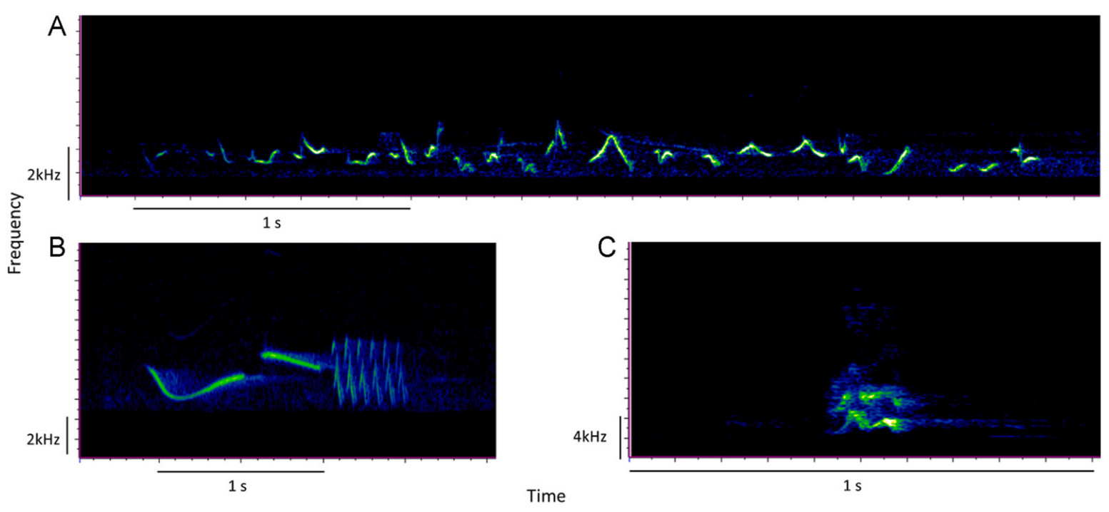
 DownLoad:
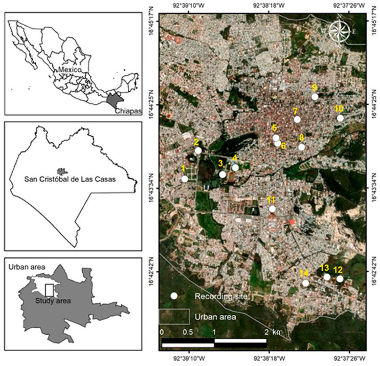
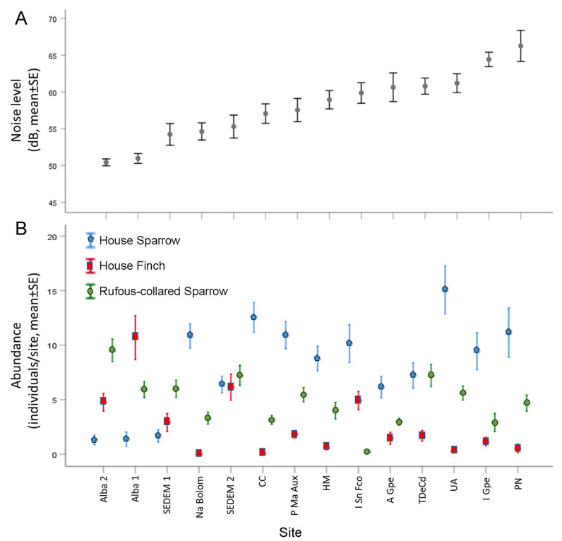

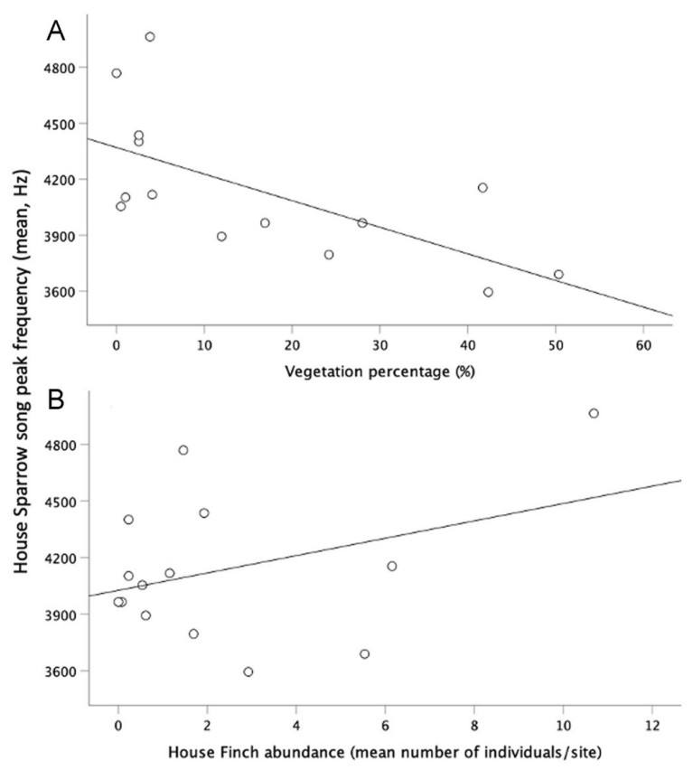
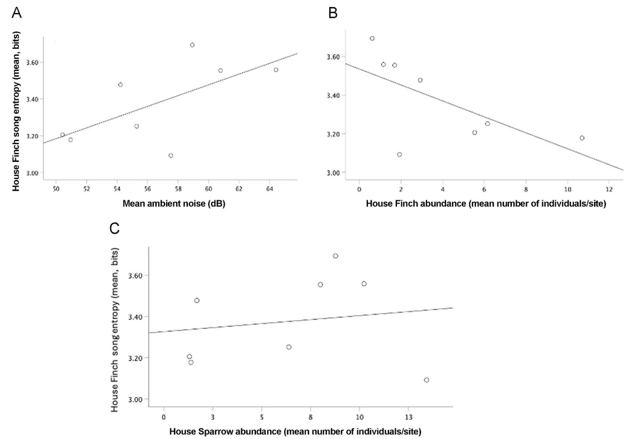
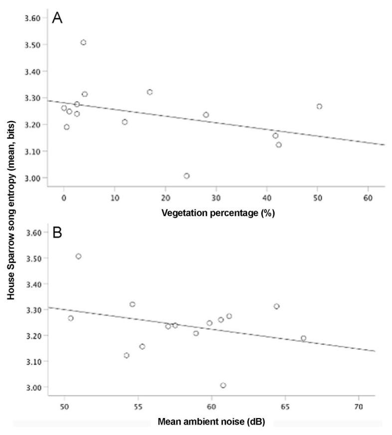
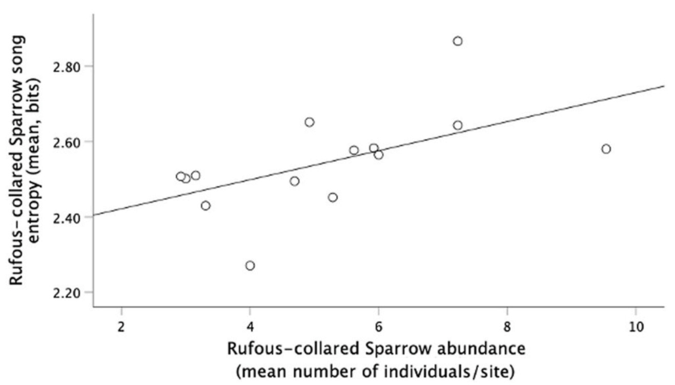


 Email Alerts
 RSS Feeds