Jian Ding, Shengnan Wang, Wenzhi Yang, Huijie Zhang, Ni Wang, Yingmei Zhang. 2025: How does asymmetric sibling rivalry respond under environmental metal pollution? A case study of the Tree Sparrow (Passer montanus). Avian Research, 16(1): 100225. DOI: 10.1016/j.avrs.2025.100225
Citation:
Jian Ding, Shengnan Wang, Wenzhi Yang, Huijie Zhang, Ni Wang, Yingmei Zhang. 2025: How does asymmetric sibling rivalry respond under environmental metal pollution? A case study of the Tree Sparrow (Passer montanus). Avian Research, 16(1): 100225. DOI: 10.1016/j.avrs.2025.100225
Jian Ding, Shengnan Wang, Wenzhi Yang, Huijie Zhang, Ni Wang, Yingmei Zhang. 2025: How does asymmetric sibling rivalry respond under environmental metal pollution? A case study of the Tree Sparrow (Passer montanus). Avian Research, 16(1): 100225. DOI: 10.1016/j.avrs.2025.100225
Citation:
Jian Ding, Shengnan Wang, Wenzhi Yang, Huijie Zhang, Ni Wang, Yingmei Zhang. 2025: How does asymmetric sibling rivalry respond under environmental metal pollution? A case study of the Tree Sparrow (Passer montanus). Avian Research, 16(1): 100225. DOI: 10.1016/j.avrs.2025.100225
School of Life Sciences, Henan Normal University, Xinxiang, 453007, China
b.
Gansu Key Laboratory of Biomonitoring and Bioremediation for Environmental Pollution, School of Life Sciences, Lanzhou University, Lanzhou, 730000, China
Funds:
the National Natural Science Foundation of China32370508
the National Natural Science Foundation of China32201266
the China Postdoctoral Science FoundationGZC20230731
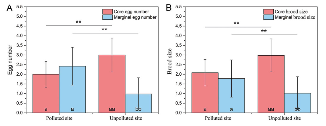
The imbalanced allocation of maternal resources to eggs and nestlings may significantly impact the phenotype and fitness of offspring. Moreover, anthropogenic metal pollution has been reported to exert adverse effects on avian offspring. Therefore, we herein evaluated the relationships among offspring characteristics, asymmetric sibling rivalry, and the resulting offspring phenotype in a small passerine bird, Tree Sparrow (Passer montanus), at a polluted site (Baiyin, BY) and a relatively unpolluted site (Liujiaxia, LJX). By initiating incubation before the completion of clutch, asymmetric sibling rivalry might create a core and marginal offspring within the brood. In this study, lower egg mass, fewer core offspring, and more marginal offspring were found at the polluted site. Although eggshell speckling and coloration were relatively similar between the two sites, higher eggshell spotting coverage ratio and lower eggshell lightness (L*) and hue (h°) were observed in core eggs than in marginal eggs at the unpolluted site. The clutch size had a positive relationship with egg mass at the polluted site and with brood size at hatching at the unpolluted site. The differences in egg measurements across the laying orders in the samples were relatively large for larger clutch sizes. The core and marginal egg masses had a significant positive effect on the size of early core nestlings and late marginal nestlings at the unpolluted site. Fledgling rate was significantly positively related to the incubation period and nestling period, while negative relationship with mean spotting coverage ratio was found at the polluted site. Marginal nestlings at the polluted site showed a higher mortality rate. Overall, although asymmetric sibling competition strongly determines the variation of marginal offspring size, the effect is less dramatic in metal-polluted environments, providing some respite to wild birds that survive pollution-induced stress.
Wetlands are crucial ecosystems that provide various ecological services and support a wide range of biodiversity. They are characterized by a unique combination of aquatic and terrestrial features, making them highly productive and biologically diverse (Mitsch et al., 2009). However, wetlands worldwide are experiencing a rapid degradation in quality and significant reduction in area as a result of human activities and environmental changes, e.g., urbanization, agricultural expansion, wetland filling and drainage, changes in water resource management, land development, and sea-level rise caused by climate change (Herbert et al., 2015; Xu et al., 2019). Until now, there has been a 35% reduction in the global wetland extent since 1970, according to the Ramsar Convention on Wetlands (2018). Concurrently, wetland functions and services have undergone changes, posing significant threats to their ecological integrity and the species dependent on them (Engelhardt and Ritchie, 2001). Therefore, understanding the impact of wetland degradation on biodiversity is essential for effective conservation and management strategies.
Birds, being highly responsive to environmental changes and having specific habitat requirements, serve as excellent indicators of wetland health and ecosystem functioning. They play vital roles as pollinators, seed dispersers, and regulators of insect populations, making them valuable indicators of overall wetland ecosystem health (Robledano et al., 2010; Fraixedas et al., 2020). Previous studies have made significant progress in investigating the negative effects of wetland degradation on bird species diversity and have utilized birds as indicators of wetland degradation (Brazner et al., 2007; Mistry et al., 2008). However, the field of research on wetland degradation and its impact on avian diversity faces several significant challenges and shortcomings that require further interdisciplinary investigation for resolution. Firstly, the negative impacts of reclamation and agricultural expansion on wetland ecosystems have received attention, but there is still limited research on the long-term cumulative effects of specific human activities, such as wetland development and pollution, and the mechanisms underlying bird community responses to these disturbances (Zou et al., 2018; Luo et al., 2019; Dong et al., 2022). We need to move beyond localized studies and consider the influence of wetland degradation on avian diversity across different geographical units, accounting for variables such as altitude, climate, and anthropogenic activities (Mekonnen and Aticho, 2011; Sebastian-Gonzalez and Green, 2016). Secondly, existing research predominantly focuses on avian diversity during a specific period, such as the breeding or wintering seasons, leaving a critical gap in understanding seasonal variations and their impact on avian diversity. For instance, previous studies on waterbirds in the Zoige Wetlands have primarily concentrated on the breeding season (Xu et al., 2021; Yang and Chen, 2024), with limited continuous monitoring of wintering waterbirds, as observed in the middle and lower Yangtze wetlands (Luo et al., 2019; Wang et al., 2020). Comparative analyses of bird community structures across different time periods are essential to gain a clearer understanding of the role wetland ecosystems play in supporting bird population throughout their entire life cycle. Additionally, in terms of research methods and indicators, past studies have primarily employed traditional bird metrics and indices to measure avian diversity, such as species richness, abundance, and taxonomic composition (Fang et al., 2006; Woldemariam et al., 2018). However, emerging ecological diversity indices like phylogenetic, functional diversity, and community similarity indices offer more nuanced insights into biodiversity than traditional measures like species richness, as they account for evolutionary history and the roles species play in their ecosystems, which may be used for further exploration in the context of wetland degradation studies (Calba et al., 2014). Lastly, there is a lack of comparisons of population diversity across different stages of wetlands in various seasons, as well as quantitative indicators for selecting bird indicator species, which are crucial for understanding the co-evolution of animal groups during the succession process of wetland degradation (Ma et al., 2007). By examining these indicator species, we can gain a better understanding of animal responses under the spatiotemporal patterns of wetland degradation, then investigate the specific mechanisms and ecological processes underlying the interplay between wetland degradation and other potential disturbance factors, furthermore provide valuable insights and recommendations for local government conservation strategies and policies (Siddig et al., 2016).
The Zoige Alpine Wetland Ecosystem, located on the northeastern edge of the Qinghai-Tibet Plateau, is currently the world's largest high-altitude marsh distribution area and the largest peat storage area in China (Bai et al., 2008; Xu et al., 2021). The region's unique geological, climatic, and hydrological conditions provide an exceptional environment for the survival and reproduction of rare wildlife and plants, making it a hotspot for global biodiversity research. It is listed as an internationally important wetland under the Ramsar Convention and is recognized as a biodiversity hotspot (Yang, 2007). Additionally, the marsh and peat layers in the Zoige Plateau Wetland area have enormous water retention and storage capacity, with a total water storage of nearly 10 billion m3. This area serves as a vital water source supply zone for the upstream regions of the Yangtze and Yellow Rivers. Because of this, it not only provides the foundation for local biodiversity but also ensures ecological security downstream (Tian et al., 2005). However, this pristine ecosystem is experiencing degradation due to factors such as overgrazing, land conversion, and climate change (Bai et al., 2008; Cui et al., 2015; Wu et al., 2018).
To better understand wetland ecosystems and avian diversity, as well as the relationship between them, our research was centered in the Zoige Alpine Wetland, encompassing both summer and winter seasons. We selected birds as indicator species to achieve three primary objectives within the Zoige Alpine Wetland Ecosystem's various degradation gradients: 1) to investigate the composition and distinctions in wetland bird populations across four degradation levels, employing a range of biodiversity indices encompassing taxonomic, phylogenetic, and functional diversity; 2) to evaluate the influence of wetland degradation on avian community structures during different seasons, thus shedding light on the temporal variability of wetland degradation impacts; 3) to identify potential indicator species specific to various degraded wetland stages based on our research findings, serving as valuable references for subsequent wetland monitoring and conservation efforts.
2.
Materials and methods
2.1
Study area
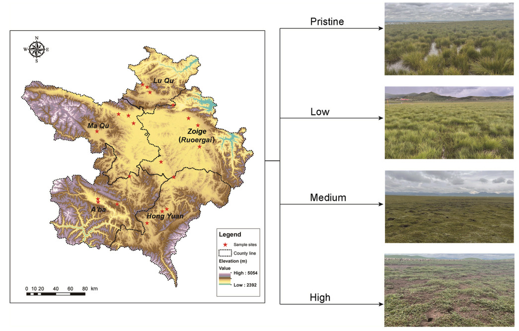
Our studies area located in the upper reaches of the Yellow River valley in the eastern part of the Qinghai-Tibet Plateau (101°50′ to 103°39′ E and 32°56′ to 34°19′ N). The elevation in this region ranges from 3400 to 3900 m. Zoige Wetland covered five counties, with a total area of 19, 600 km2 (Fig. 1). This area experiences a high-altitude cold temperate monsoon climate, characterized by a yearly average temperature ranging from 0.96 ℃ to 2.2 ℃. The hottest month is July, with an extreme maximum temperature of 24.6 ℃, while the coldest month is January, with an extreme minimum temperature of −33.6 ℃. Precipitation is concentrated mainly from May to August, gradually decreasing from south to north. The annual average precipitation varies between 600 mm and 800 mm, while the annual average evaporation ranges from 1200 mm to 1500 mm. The region enjoys ample sunshine and strong solar radiation, with an annual frost-free period of fewer than 100 days. The core area of the wetland is comprised of lakes, marshes, and rivers, and soil types are predominantly alpine meadow soil and subalpine meadow soil, with marsh soil and peat soil distributed secondarily (Cui et al., 2015).
Figure
1.
Bird sampling sites and four degraded level wetlands in Zoige Plateau. Details for four degraded level classifieds were given in the section Materials and methods.
We delineated four distinct degradation gradients within plateau wetlands, as per the criteria established in previous literature. We first used satellite remote sensing maps (Google Earth) to visually assess wetland degradation and select candidate sampling sites. Within each site type, five 50 cm × 50 cm quadrats were randomly chosen, where species richness was recorded, and total community coverage and water accumulation were estimated. Finally, we classified the degree of wetland degradation based on vegetation coverage, water accumulation, and dominant plant types, resulting in a comprehensive classification system (as detailed below) (Bao et al., 2021; Wang et al., 2022). Pristine Wetland: this highest quality wetland is characterized by a vegetation cover ≥90%, perennial water accumulation, and the dominant species are Carex muliensis, C. capilliformis, C. wuergaiana, Kobresia humilis, Potentilla anserina, Lysimachia paridiformis var. stenophylla, Veronica anagallis-aquatica, Equisetum ramosissimum, Trollius chinensis, Alopecurus arundinaceus, Utricularia heterosepala, Chara braunii, and Alopecurus pratensis var. japonicas. Low Degradation Wetland: vegetation cover ranging between 75% and 90%, with the occurrence of seasonal water accumulation, and the predominant species are C. muliensis, C. capilliformis, Carex wuergaiana, P. anserina, L. paridiformis var. stenophylla, K. tibetica, and Pedicularis densispica. Medium Degradation Wetland: characterized by a vegetation cover of 50%–75%, this gradient lacks extensive water accumulation but features small water pits and moist soil surfaces, and the dominant species are Medicago sativa, K. pygmaea, Ranunculus tanguticus, L. paridiformis var. stenophylla, Poa annua, Stipa breviflora, Artemisia frigida, and Artemisia sphaerocephala. High Degradation Wetland: the most degraded type, with vegetation cover ≤50% or less and perennial absence of water accumulation, and the dominant species are C. atrata, Oxytropis kansuensis, K. humilis, Leontopodium dedekensii, P. kansuensis, Ulmus pumila var. sabulosa, Lonicera hispida, C. arenaria, and Chrysanthemum leucanthemum. Each of these habitat types is visually represented in Fig. 1, informed by data meticulously collected during our survey.
2.3
Bird surveys
The Zoige Wetland is mainly distributed in Ruoergai County, Hongyuan County, Aba County in Sichuan Province, and Luqu County and Maqu County in Gansu Province; thus, five sampling areas were selected across Zoige Wetland. At each county, we selected four types of wetland degradation habitats. Then, within each degradation level, we randomly chose one transect, resulting in a total of 20 transects (5 transect lines for each degradation gradient) (Fig. 1). The relatively limited number of selected transects (20 in total) may introduce some variability in the data. Given the extensive area of the wetland and the considerable spatial distances between transects, we adopted a systematic sampling approach to ensure adequate representation, thereby facilitating comprehensive coverage and supporting reliable data collection. We conducted standard transect surveys to assess breeding and summer migrant bird populations across 20 transect lines in June 2022 (Appendix Table S1). These surveys, covering 20 transect lines, were repeated to evaluate resident and winter migrant bird communities in November 2022. Each transect line was 1–3 km in length, with no overlap between transects and a minimum interval of 2 km between them.
During the surveys, observations were primarily made using binoculars (Zeiss 8 × 42), supplemented by sound identification and photographic evidence. Survey teams, consisting of 2–3 observers, walked at a uniform speed of 2 km/h, recording the species and number of birds seen or heard within a 50–100 m range on either side of the transect. Considering the variation in visibility due to differing vegetation covers among degradation levels, observer movement during transect surveys, which can increase the detection rates of small and elusive bird species. All recorded bird calls and songs were identified to species level using a combination of visual and auditory cues based on standard field guides (Bibby, 2000; Zheng, 2017).
2.4
Phylogenetic, functional dendrogram and heatmap analysis
To obtain the phylogenetic tree, we pruned the global phylogenetic tree of birds from BirdTree (http://birdtree.org) under the option of 'Hackett All Species: a set of 10, 000 trees with 9993 OTUs each' to include 106 birds from this study (Jetz et al., 2014). We then sampled 5000 pseudo-posterior distributions and constructed the Maximum Clade Credibility tree using mean node heights by the software TreeAnnonator v2.6.6 of the BEAST package (Drummond and Rambaut, 2007; Ricklefs and Jønsson, 2014). We used this resulting tree for all subsequent analyses on phylogenetic analyses (Appendix Fig. S1A). To establish the trait tree, we initially examined various functional traits, including body mass (g), wing length (cm), diet, nest site, and residential type, which have been extensively studied in previous works (Si et al., 2017; Liang et al., 2019). These traits are particularly crucial as they are closely associated with resource requirements and habitat preferences (Ding et al., 2013). Our functional data were gathered through comprehensive fieldwork and an extensive review of the literature (Zhao, 2001; Wilman et al., 2014). Diet was classified as (1) omnivore, (2) herbivore, (3) carnivore, and (4) scavenger, while nest sites were categorized as (1) cavity, (2) tree, (3) shrub, (4) water, and (5) ground. Additionally, the residential type was divided into (1) resident, (2) summer visitor, (3) winter visitor, (4) passage migrant, and (5) vagrant visitor (Appendix Table S2). Gowdis function converted functional traits into a distance matrix. Subsequently, the Gower distance matrix underwent hierarchical clustering utilizing the hclust function, with the "average" linkage method applied to derive a dendrogram illustrating the dissimilarities among functional traits. This hierarchical clustering output was then converted into a phylogenetic tree using the as.phylo function, finalizing the construction of the functional dendrogram (Appendix Fig. S1B).
2.5
Taxonomic, phylogenetic, functional diversity and similarity
For diversity estimation, we employed the Shannon diversity index to assess taxonomic diversity (TD), utilizing the 'diversity' function within the vegan package. We then calculated the total branch length occupied by all species within a local community's phylogenetic tree for estimation the Phylogenetic Diversity (PD) by 'PD' function in the picante package. Additionally, we evaluated Functional Diversity (FD) through the 'gowdis' function within the 'FD' package (Faith, 1992). For similarity estimation, we utilized the Sørensen index to evaluate taxonomic similarity, which measures the proportion of shared species relative to the total number of species present in two assemblages. Taxonomic community similarity (TDSI) was computed using the 'betadiver' function within the vegan package (Soininen et al., 2007; Oksanen, 2011). For assessing phylogenetic community similarity (PDSI) between transects within each degraded levels over time, we employed the Phylosor index. The Phylosor index quantifies the proportion of shared branch length in relation to the total evolutionary branch length between two samples (Feng et al., 2012). Additionally, we determined functional community similarity (FDSI) using the Phylosor index based on the functional dendrogram. Phylogenetic and functional similarities were calculated using the 'phylosor' function within the 'picante' package (Kembel et al., 2010). To compare the differences in bird diversity across wetlands with varying degrees of degradation, we calculated the Jaccard dissimilarity index based on the number of species within the same order for each wetland, using the 'vegdist' function from the Vegan package. The Jaccard index ranges from 0 to 1, where 1 indicates complete dissimilarity in the species composition of the two degraded level wetlands, and 0 indicates complete similarity (Chase et al., 2011).
The standardized effect size (SES) of phylogenetic and functional similarities for each assemblage was calculated to eliminate the influence of taxonomic similarities. The SES for phylogenetic similarity (SESphylosor) was computed as follows:
where Phylosorobs represents the observed phylogenetic or functional 'Phylosor' similarities of bird communities between two transects within each habitat. The mean Phylosorrnd denotes the mean 'Phylosor' similarities derived from null models (which involve shuffling species labels in community data while maintaining species richness and shared species between communities across 999 iterations), and sd Phylosorrnd is the standard deviation of 'Phylosor' similarities from these null models.
2.6
Indicator species analysis
We performed indicator species analysis to identify bird species associated with degradation level wetland using the indicspecies package in R (De Caceres et al., 2016). This analysis aimed to identify species that serve as indicators for specific habitat conditions or seasonal groupings. Bird species abundance data were categorized by wetland degradation levels (pristine, low, medium, high) and seasons (winter, summer). The Group variable, which combined degradation levels and seasons, was used to define the classification of sampling sites into groups. Data matrices included bird species abundances as rows and sampling sites as columns, ensuring compatibility for analysis. The function 'multipatt' was used to compute indicator values (IndVal) for species-site group associations. A permutation test with 999 permutations was performed to assess the statistical significance of these associations. The stat value quantifies the strength of association between a species and a specific environment or group. The stat value of 1 indicates a strong association, with the species showing high frequency and abundance in the group, almost serving as an indicator. A stat value close to 0 indicates a weak association, with low frequency or abundance in the group. Specificity (Component A), which measures the probability that a site belongs to a particular group given the presence of the species, reflects its positive predictive value as an indicator; and Fidelity (Component B), which measures the probability of finding the species in sites belonging to the group, represents its sensitivity as an indicator (Cáceres and Legendre, 2009).
2.7
Statistical analysis
All continuous variables were tested for normality using the Kolmogorov–Smirnov test and transformed variables were tested when needed to meet the assumptions of ANOVA analysis. To examine the impact of seasonal variations and degree differences on the biodiversity indices, we performed two-way ANOVA to compare the difference in TD, PD and FD values among four degraded groups and seasons. We first set TD, PD and FD values as dependent variables, then set the degraded degree with four levels (pristine, low, medium and high) and season with two levels (summer and winter) as the independent variables. The interaction term (Degradation × Season) was selected to determine if TD, PD and FD value in different degraded wetlands changed betwee seasons in the same pattern. If the interaction term is significant (P < 0.05), it indicates that these indices are affected by seasonality. Tukey's honestly significant difference (HSD) test was conducted for post-hoc comparisons between all combinations of any two season and degraded groups. All results were considered significant if P < 0.05. All statistical analyses were performed using R Core Team ver. 4.2.1.
3.
Results
3.1
Species composition in wetlands of varying degradation levels across different seasons
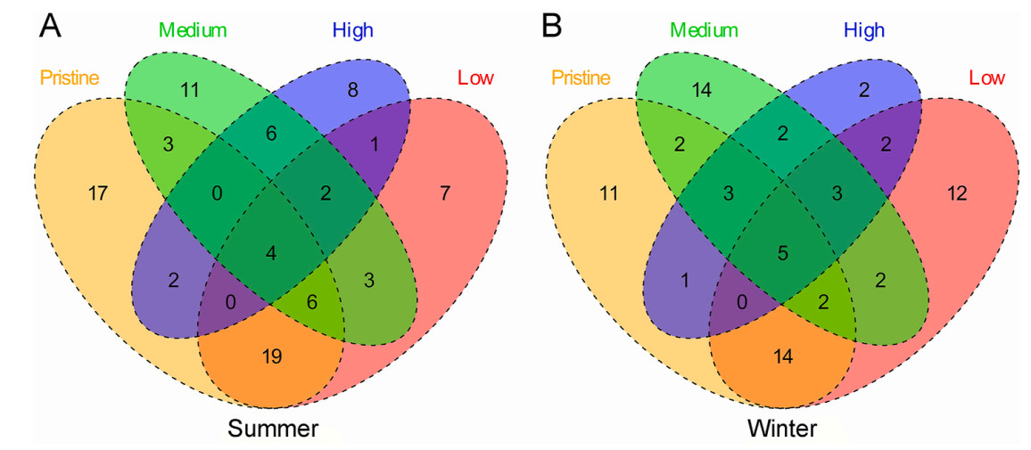
A total of 106 bird species from 32 families and 14 orders were observed in Zoige Wetlands. Among all bird species, Passeriformes represented the predominant order, comprising 51 species, constituting 48.11% of the total. Anseriformes order encompassed 17 species, equivalent to 16.04% of the population. Additionally, Accipitriformes accounted for 10 species, constituting 9.43% (Appendix Table S3). Focusing on individual species, Passer montanus accounted for the largest number of counted individuals (241 records, 12.24%), followed by Tadorna ferruginea (145 records, 7.36%), Onychostruthus taczanowskii (108 records, 5.49%), and Netta rufinai (92 records, 4.67%). The Venn diagrams depict varying distributions and overlaps of avian species under different disturbance levels and seasons. We observed that the number of species decreased with increasing disturbance levels in both winter and summer, with a higher number of species overlap occurring between groups with similar disturbance levels (Fig. 2). Moreover, we found that both 'pristine' and 'low' disturbance levels exhibited the greatest overlap of avian species in summer (29 species) and winter (21 species). Nevertheless, with the rise in disturbance levels categorized as 'medium' and 'high', there was a decline in species overlap, with only 12 species in summer and 13 species in winter.
Figure
2.
Birds species overlap among four degraded level wetlands, illustrated by a Venn diagram representing the number of species recorded in summer (A) and winter (B).
3.2
Degrade and seasonal effect for diversity index
We controlled for the season effect by including it as a factor in the two-way ANOVA, and observed that the significant differences in TD, PD, and FD across wetland degradation levels were independent of seasonal variations (P < 0.01; Table 1). Additionally, post hoc analysis indicated that the 'pristine' and 'low' degraded groups exhibited higher values for TD, PD and FD compared to the 'high' and 'medium' groups (P < 0.05) (Fig. 3A). Taxonomic, phylogenetic and functional similarities were also explained by degraded levels (two-way ANOVA: P < 0.05; Table 1). From summer to winter, PD exhibited an increase (two-way ANOVA: F = 18.00, P < 0.05); in contrast, TD and FD showed no significant seasonal differences. Furthermore, no significant interaction between season and degradation level for TD and FD (Fig. 3A, Table 1) suggests that these indices are similarly affected by seasonality. However, this pattern was not observed for PD, where the interaction between season and degradation level was significantly different (F = 14.69, P < 0.01).
Table
1.
Two-way ANOVA results for the effects of degradation, season and their interactions on the taxonomic, phylogenetic and functional diversity index and community similarities.
Diversity index
Degradation
Season
Degradation season
F
P
F
P
F
P
TD
20.95
< 0.01
3.86
0.05
1.47
0.24
PD
49.56
< 0.01
18.00
< 0.01
4.69
< 0.01
FD
22.45
< 0.01
2.24
0.14
0.22
0.87
TDSI
10.17
< 0.01
2.12
0.15
2.74
0.04
PDSI
3.74
< 0.05
2.18
0.14
0.64
0.58
FDSI
4.18
< 0.01
2.93
0.09
4.01
< 0.05
Note: TD: taxonomic diversity; PD: phylogenetic diversity; FD: functional diversity; TDSI: taxonomic community similarity; PDSI: phylogenetic community similarity; FDSI: functional community similarity.
Figure
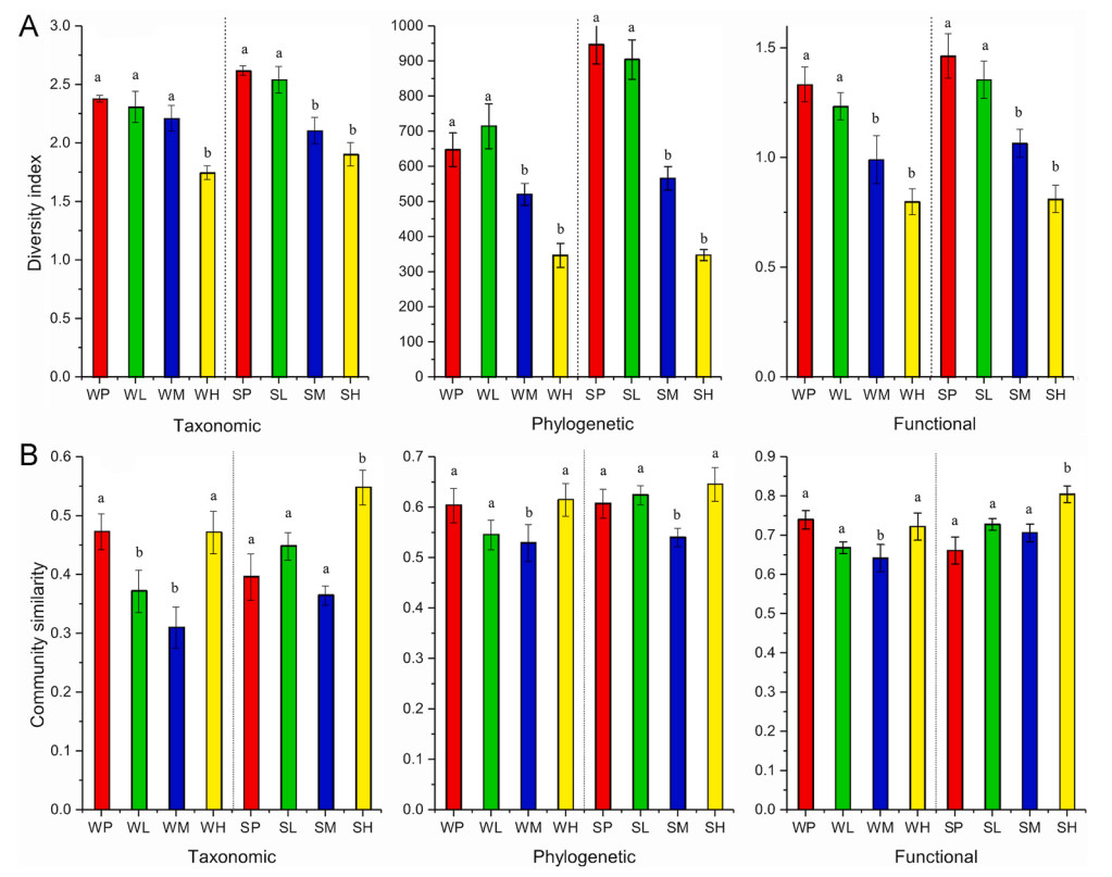
3.
Results of Tukey's multiple comparisons for the taxonomic, phylogenetic and functional diversity index (A) and community similarities (B) of bird in four degraded groups (P: pristine, L: low, M: medium and H: high) between summer (S) and winter (W) seasons in Zoige Wetland.
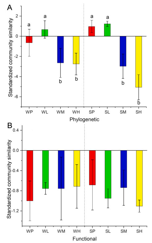
Community similarities were explained by degraded levels (TDSI: F = 10.17, P < 0.01; PDSI: F = 3.74, P < 0.05; FDSI: F = 18.00, P < 0.01), but not explained by season (P > 0.05) (Table 1). Post hoc analysis revealed that in the winter, TDSI, PDSI and FDSI values for the pristine and high disturbance groups exhibited higher community similarities compared to the low and medium degraded groups. However, in the summer, the TDSI, PDSI and FDSI values did not show consistent patterns, with the three indices displaying different trends of variation (Fig. 3B). For SES phylogenetic similarities, medium and highly degraded wetlands tended to have lower similarities compared to pristine and low-degraded wetlands, whereas no significant differences were observed in SES functional similarities (Fig. 4).
Figure
4.
Results of Tukey's multiple comparisons for the standardized effect size (shuffle species labels in community data while maintain species richness and species shared between communities for 999 times) of phylogenetic (A) and functional (B) similarities of bird communities in four degraded groups (P: pristine; L: low; M: medium; and H: high), based on linear mixed effects models.
3.3
Indicator species for wetlands at various degradation levels across different seasons
In summer, 13 bird species were identified as being significantly associated with varying levels of wetland degradation. In pristine wetlands, the Common Sandpiper (stat = 0.78, P < 0.05) was the only species significantly associated. In high degradation wetlands, two species were significantly associated: the Rufous-necked Snowfinch (stat = 0.91, P < 0.01) and the Horned Lark (stat = 0.78, P < 0.05). In winter, 12 bird species were identified for the indicator species. In pristine wetland, four species were significantly associated, namely the Bar-headed Goose (stat = 0.99, P < 0.01), Red-crested Pochard (stat = 0.89, P < 0.01), Common Goldeneye (stat = 0.78, P < 0.05), and Northern Pintail (stat = 0.74, P < 0.05). In low degradation wetlands, only one species, Ferruginous Pochard (stat = 0.99, P < 0.01), was significantly associated. In medium degradation wetlands, Red-billed Chough (stat = 0.80, P < 0.05) was the only species significantly associated with this group. In high degradation wetlands, White-rumped Snowfinch (stat = 0.83, P < 0.05) was significantly associated (Table 2).
Table
2.
Indicator species analysis for bird species associated with different wetland degradation levels during winter and summer.
Season
Group
Common name
Scientific name
A
B
stat
P
Winter
Group 1
Bar-headed Goose
Anser indicus
0.98
1.00
0.99
< 0.01
Winter
Group 1
Red-crested Pochard
Netta rufina
0.99
0.80
0.89
< 0.01
Winter
Group 1
Common Goldeneye
Bucephala clangula
1.00
0.60
0.78
< 0.05
Winter
Group 1
Northern Pintail
Anas acuta
1.00
0.60
0.78
< 0.05
Winter
Group 2
Ferruginous Pochard
Aythya nyroca
0.69
0.80
0.74
< 0.05
Winter
Group 3
Red-billed Chough
Pyrrhocorax pyrrhocorax
0.80
0.80
0.80
< 0.05
Winter
Group 4
White-rumped Snowfinch
Onychostruthus taczanowskii
0.69
1.00
0.83
< 0.05
Winter
Group 1+2
Ruddy Shelduck
Tadorna ferruginea
0.95
1.00
0.97
< 0.01
Winter
Group 1+2
Mallard
Anas platyrhynchos
0.97
0.90
0.94
< 0.01
Winter
Group 1+2
Black-headed Gull
Larus ridibundus
1.00
0.80
0.89
< 0.05
Winter
Group 1+2
Brown-headed Gull
Larus brunnicephalus
1.00
0.70
0.84
< 0.05
Winter
Group 1+2
Common Merganser
Mergus merganser
0.96
0.70
0.82
< 0.05
Winter
Group 1+3+4
Eurasian Tree Sparrow
Passer montanus
0.99
0.73
0.85
< 0.05
Summer
Group 1
Common Sandpiper
Actitis hypoleucos
1.00
0.60
0.78
< 0.05
Summer
Group 4
Rufous-necked Snowfinch
Pyrgilauda ruficollis
0.82
1.00
0.91
< 0.01
Summer
Group 4
Horned Lark
Eremophila alpestris
1.00
0.60
0.78
< 0.05
Summer
Group 1+2
Ruddy Shelduck
Tadorna ferruginea
1.00
1.00
1.00
< 0.01
Summer
Group 1+2
Common Coot
Fulica atra
0.92
1.00
0.96
< 0.01
Summer
Group 1+2
Ferruginous Pochard
Aythya nyroca
1.00
0.80
0.89
< 0.01
Summer
Group 1+2
Common Redshank
Tringa totanus
1.00
0.80
0.89
< 0.01
Summer
Group 1+2
Little Egret
Egretta garzetta
0.96
0.80
0.88
< 0.05
Summer
Group 1+2
Little Grebe
Tachybaptus ruficollis
1.00
0.60
0.78
< 0.05
Summer
Group 1+2
Mallard
Anas platyrhynchos
1.00
0.60
0.78
< 0.05
Summer
Group 3+4
White-rumped Snowfinch
Onychostruthus taczanowskii
1.00
0.90
0.95
< 0.01
Summer
Group 3+4
Oriental Skylark
Alauda gulgula
0.95
0.70
0.82
< 0.05
Note: The Season column indicates whether the data corresponds to winter or summer. The Group column refers to the specific wetland degradation level, such as Group 1 (Pristine), Group 2 (Low degradation), Group 3 (Medium degradation), and Group 4 (High degradation). The explanations of parameters A, B, and stat are provided in Section 2.6.
In both winter and summer, the Jaccard index exhibited consistent patterns, with species similarity divided into two groups. Jaccard index was lower between pristine and low-degraded wetlands (0.35–0.54) and higher between medium- and high-degraded wetlands (0.08–0.21). The lowest species similarity was observed between pristine and high-degraded wetlands (0.83–0.89) (Table 3).
Table
3.
Beta diversity index of wetlands with different degrees of degradation based on the Jaccard coefficient matrix. Jaccard dissimilarity index was calculated using the number of species within the same family for each wetland level.
Our study found that avian communities have more shared species and exhibit higher community similarity between adjacent successional gradients (Fig. 2), indicating continuity in community structure across different stages of wetland degradation and succession. This result suggests that the current avian community structure in a given region is influenced by the complex interaction of environmental factors and the dynamic processes of succession. This pattern of community succession has been observed in other ecosystems as well. For instance, previous studies on secondary forest succession have shown transitional changes in the diversity and composition of amphibians, reptiles, birds, and mammals (Acevedo-Charry and Aide, 2019). Similarly, research on wetland degradation has highlighted analogous transitional shifts in avian communities, with the inheritance of community structure evident across different degradation stages (Xu et al., 2021).
Our findings underscore the multifaceted nature of the impact of wetland degradation on avian community dynamics. Specifically, our study reveals that Zoige Wetlands undergo successive stages of degradation, leading to discernible shifts in species composition, abundance, and diversity among avian populations (Table 1). As wetland degradation increased, we observed shifts in the dominant bird species, changes in species richness, and alterations in avian functional and phylogenetic diversity (Fig. 3A). Community similarity analysis revealed that TDSI, PDSI, and FDSI values were lower in the low and medium-degraded wetlands compared to the pristine and high degraded groups (Fig. 3B). However, as the wetland underwent degradation, experiencing reduced water levels and vegetation changes, it transformed into an environment with less water and increased grassland coverage with higher similarity in TDSI, PDSI and FDSI. The Jaccard index similarly indicates that this transition from pristine wetlands to degraded stages has been linked to the most significant shifts in bird species composition (Table 2), reflected in a decrease in the abundance of specific waterbird and shorebird species. Conversely, some terrestrial and generalist species (Eurasian Tree Sparrow Passermontanus, Oriental Skylark Alauda gulgula, White-rumped Snowfinch Onychostruthus taczanowskii, and Red-necked Snow Finch O. ruficollis) have tended to become more dominant and widespread in highly degraded wetlands. Additionally, a previous study suggests that in highly degraded wetlands, rodent species and Passeriformes may engage in mutual vigilance behavior to evade predators, such as raptors (Rosvold, 2016).
4.2
Season effects
Seasonal dynamics also play a pivotal role in shaping avian community structures within wetlands, particularly when considering their interactions with varying levels of wetland degradation (Panda et al., 2021; Htay et al., 2023). Previous study speculated this influence was attributed to two primary factors: the distinct ecological requirements and behavioural patterns of different avian groups and the seasonal influx of migratory birds (Tu et al., 2020; Donnelly et al., 2021). Our data support that degraded degree was significant effect on PD across seasons, but TD and FD were not different between two seasons (Table 1, Fig. 3A). During the breeding season, wetland degradation often leads to habitat loss, water quality deterioration, and vegetation disruption. These alterations can result in the loss of suitable nesting sites and food resources for breeding birds, causing a decline in species diversity (Żmihorski et al., 2016; Gao et al., 2021). For example, water-associated bird species like Black-necked crane (Grus nigricollis) and Common Coot (Fulica atra) suffered from water depth and vegetation coverage decreasing, as their breeding nest need concealment for avoid predator and human disturbance in breeding season (Jiang et al., 2017; Xiao et al., 2017). Moreover, Zoige serves as a crucial stopover and overwintering site within the migratory route of China, connecting regions from Russia, Mongolia, the western Tibetan Plateau, and extending to Southeast Asia (Zhang et al., 2014). The migratory activities of birds during the winter season, involving arrivals and departures, exert a profound influence on the composition and structure of avian communities, distinct from the breeding season. Consequently, the impact of wetland degradation tends to be more pronounced during the winter season, which aligns with the findings from our data.
However, it is essential to note that the effect of seasonal changes varies significantly across wetlands with different degrees of degradation (Table 1). Our results show that low and medium degraded wetlands exhibit lower community similarity. Compared to the highest species diversity in pristine wetlands and the lowest in highly degraded wetlands (Fig. 3, Fig. 4), the varying levels of disturbance in low and medium degraded wetlands create habitat heterogeneity, changes in predation pressure, diversification of food resources, and impacts from climate change, among other factors (Brooks et al., 2005). This heterogeneity may provide the necessary conditions for a wider range of bird species, resulting in lower community similarities at these two stages. However, once wetlands degrade to a highly degraded state, the extremely low number of bird species and populations lead to a high degree of community similarity, making it more difficult to reverse the degradation and restore ecosystem functions and services (Sebastian-Gonzalez and Green, 2016; Xu et al., 2019). Therefore, addressing the intermediate stages of wetland degradation is crucial for conserving wetland bird diversity.
4.3
Indicator species
Birds are ideal indicator species due to their sensitivity, ease of monitoring, and high public awareness (Fraixedas et al., 2020). By establishing local bird species databases and continuously monitoring avian community dynamics, including metrics such as species richness, Shannon diversity indices, phylogenetic and functional diversity, we can gain valuable insights into changing environmental trends and the overall health of ecosystems. We attempt to explore the relationship between wetland degradation and bird species diversity, identifying suitable bird species to indicate wetland degradation processes and wetland quality. Our results demonstrate that degraded wetlands exhibit different indicator species across seasons, reflecting the seasonal variation in how wetland resources, such as food availability, shelter, and resting areas, are utilized by different bird species (Table 1). We found that smaller-bodied species are more sensitive to wetland degradation. For instance, during the summer, sandpipers were identified as indicator species for pristine wetlands. However, as wetlands underwent low degradation, larger-bodied species, such as Northern Pintail and Mallard, emerged as indicator species. When wetlands experienced further degradation, passerine birds such as sparrows, snow finches, and larks became predominant. Additionally, there was an increasing prevalence of raptors, such as the Red-billed Chough, which signifies medium to high degradation of high-altitude wetlands (Table 2).
Furthermore, both the IndVal index (Table 2) and the Jaccard coefficient matrix (Table 3) reveal two major clusters of degraded wetlands during summer and winter: (1) pristine and low-degraded wetlands and (2) medium and high-degraded wetlands. Within each cluster, we observed greater species similarity and consistent indicator species, while significant differences were evident between the two clusters. These findings highlight the profound impact of wetland degradation on bird community composition and functional groups, underscoring the sensitivity and adaptive strategies of birds to changes in wetland resources under varying levels of degradation. Birds are particularly well-suited as indicator species for wetland degradation because of their sensitivity to changes in wetland environments (Luo et al., 2019; Panda et al., 2021). Understanding bird responses to wetland degradation is essential for guiding targeted conservation efforts aimed at mitigating its adverse effects on wetland ecosystems. We hope that this study, which correlates with different seasons and varying wetland degradation conditions, can serve as an example and provide references for future monitoring and management of wetland conditions.
The authors declare that they have no known competing financial interests or personal relationships that could have appeared to influence the work reported in this paper.
Acknowledgements
We would like to extend our sincere thanks to Wei Zhang, E'jian Zeli, Junfen Lei and Qiucheng Huang for their help on the sample collection. We thank Dr. Xiaoyi Wang for her support on data analysis. We sincerely thank Dr. Erick Zhong for his help in improving the English writing of this manuscript.
Ali, H., Khan, E., 2018. Trophic transfer, bioaccumulation, and biomagnification of non-essential hazardous heavy metals and metalloids in food chains/webs—concepts and implications for wildlife and human health. Hum. Ecol. Risk Assess. 25, 1353–1376. .
Alleva, E., Francia, N., Pandolfi, M., De Marinis, A., Chiarotti, F., Santucci, D., 2006. Organochlorine and heavy-metal contaminants in wild mammals and birds of Urbino-Pesaro province, Italy: an analytic overview for potential bioindicators. Arch. Environ. Con. Tox. 51, 123–134. .
Baird, T., Solomon, S.E., Tedstone, D.R., 1975. Localisation and characterisation of egg shell porphyrins in several avian species. Brit. Poultry Sci. 16, 201–208. .
Benton, T.G., Plaistow, S.J., Beckerman, A.P., Lapsley, C.T., Littlejohns, S., 2005. Changes in maternal investment in eggs can affect population dynamics. Proc. R. Soc. B-Biol. Sci. 272, 1351–1356. .
Bernardo, J., 1996. The particular maternal effect of propagule size, especially egg size: patterns, models, quality of evidence and interpretations. Am. Zool. 36, 216–236. .
Chevin, L.M., Lande, R., Mace, G.M., 2010. Adaptation, plasticity, and extinction in a changing environment: towards a predictive theory. PLoS Biol. 8, e1000357.
Christians, J.K., 2002. Avian egg size: variation within species and inflexibility within individuals. Biol. Rev. 77, 1–26. .
Chu, G.Z., Zheng, G.M., 1982. Feeding ecology of the tree sparrow (Passer montanus) during breeding period in the agriculture region of Beijing. Zool. Res. 3, 371–383.
Crean, A.J., Marshall, D.J., 2009. Coping with environmental uncertainty: dynamic bet hedging as a maternal effect. Philos. T. R. Soc. B. 364, 1087–1096. .
Dickens, M., Hartley, I.R., 2007. Differences in parental food allocation rules: evidence for sexual conflict in the blue tit? Behav. Ecol. 18, 674–679. .
Ding, J., Wang, S.N., Yang, W.Z., Zhang, H.J., Yu, F., Zhang, Y.M., 2023. Tissue distribution and association of heavy metal accumulation in a free-living resident passerine bird tree sparrow Passer montanus. Environ. Pollut. 316, 120547. .
Ding, J., Yang, W.Z., Wang, S.N., Zhang, H.J., Yang, Y., Bao, X.K., Zhang, Y.M., 2020. Effects of environmental metal pollution on reproduction of a free-living resident songbird, the tree sparrow (Passer montanus). Sci. Total Environ. 721, 137674. .
Ding, J., Yang, W.Z., Wang, S.N., Zhang, H.J., Zhang, Y.M., 2022. Does environmental metal pollution affect bird morphometry? A case study on the tree sparrow Passer montanus. Chemosphere 295, 133947. .
Ding, J., Yang, W.Z., Yang, Y., Ai, S.W., Bai, X.J., Zhang, Y.M., 2019. Variations in tree sparrow (Passer montanus) egg characteristics under environmental metal pollution. Sci. Total Environ. 687, 946–955. .
Dixon, L.M., Sparks, N.H.C., Rutherford, K.M.D., 2016. Early experiences matter: a review of the effects of prenatal environment on offspring characteristics in poultry. Poultry Sci. 95, 489–499. .
Eeva, T., Ahola, M., Lehikoinen, E., 2009. Breeding performance of blue tits (Cyanistes caeruleus) and great tits (Parus major) in a heavy metal polluted area. Environ. Pollut. 157, 3126–3131. .
Eeva, T., Lehikoinen, E., 1995. Egg shell quality, clutch size and hatching success of the great tit (Parus major) and the pied flycatcher (Ficedula hypoleuca) in an air pollution gradient. Oecologia 102, 312–323. .
Forbes, S., 2009. Portfolio theory and how parent birds manage investment risk. Oikos 118, 1561–1569. .
Forbes, S., Thornton, S., Glassey, B., Forbes, M., Buckley, N.J., 1997. Why parent birds play favourites. Nature 390, 351–352.
Forbes, S., Wiebe, M., 2010. Egg size and asymmetric sibling rivalry in red-winged blackbirds. Oecologia 163, 361–372. .
Glassey, B., Forbes, S., 2002. Begging and asymmetric nestling competition. In: Wright, J., Leonard, M.L. (Eds.), Evolution of Nestling Begging: Competition, Cooperation and Communication. Kluwer, Dordrecht, pp. 269–281.
Gosler, A.G., Higham, J.P., James Reynolds, S., 2005. Why are birds' eggs speckled? Ecol. Lett. 8, 1105–1113. .
Hall, M.E., Blount, J.D., Forbes, S., Royle, N.J., 2010. Does oxidative stress mediate the trade‐off between growth and self‐maintenance in structured families? Funct. Ecol. 24, 365–373. .
Hargitai, R., Nagy, G., Herényi, M., Török, J., 2013. Effects of experimental calcium availability, egg parameters and laying order on great tit Parus major eggshell pigmentation patterns. Ibis 155, 561–570. .
Hargitai, R., Nagy, G., Nyiri, Z., Bervoets, L., Eke, Z., Eens, M., Török, J., 2016. Effects of breeding habitat (woodland versus urban) and metal pollution on the egg characteristics of great tits (Parus major). Sci. Total Environ. 544, 31–38. .
Kilner, R.M., 2006. The evolution of egg colour and patterning in birds. Biol. Rev. 81, 383–406. .
Krist, M., 2011. Egg size and offspring quality: a meta‐analysis in birds. Biol. Rev. 86, 692–716. .
Kvalnes, T., Ringsby, T.H., Jensen, H., Sæther, B.-E., 2013. Correlates of egg size variation in a population of house sparrow Passer domesticus. Oecologia 171, 391–402. .
Liu, Z.P., 2003. Lead poisoning combined with cadmium in sheep and horses in the vicinity of non-ferrous metal smelters. Sci. Total Environ. 309, 117–126. .
López de Hierro, M.D.G., De Neve, L., 2010. Pigment limitation and female reproductive characteristics influence egg shell spottiness and ground colour variation in the house sparrow (Passer domesticus). J. Ornithol. 151, 833–840. .
Mainwaring, M.C., Dickens, M., Hartley, I.R., 2010. Environmental and not maternal effects determine variation in offspring phenotypes in a passerine bird. J. Evol. Biol. 23, 1302–1311. .
Martínez-Padilla, J., Dixon, H., Vergara, P., Pérez-Rodríguez, L., Fargallo, J.A., 2010. Does egg colouration reflect male condition in birds? Naturwissenschaften 97, 469–477.
Moreno, J., Osorno, J.L., 2003. Avian egg colour and sexual selection: does eggshell pigmentation reflect female condition and genetic quality? Ecol. Lett. 6, 803–806. .
Müller, W., Groothuis, T.G.G., Eising, C.M., Daan, S., Dijkstra, C., 2005. Within clutch co‐variation of egg mass and sex in the black‐headed gull. J. Evol. Biol. 18, 661–668. .
Nam, D.H., Lee, D.P., 2006. Reproductive effects of heavy metal accumulation on breeding feral pigeons (Columba livia). Sci. Total Environ. 366, 682–687. .
Orłowski, G., Hałupka, L., Pokorny, P., Klimczuk, E., Sztwiertnia, H., Dobicki, W., 2016. Variation in egg size, shell thickness, and metal and calcium content in eggshells and egg contents in relation to laying order and embryonic development in a small passerine bird. Auk 133, 470–483. .
Pan, C., Zheng, G.M., Zhang, Y.Y., 2008. Concentrations of metals in liver, muscle and feathers of tree sparrow: age, inter-clutch variability, gender, and species differences. B. Environ. Contam. Tox. 81, 558–560. .
Poláček, M., Griggio, M., Mikšík, I., Bartíková, M., Eckenfellner, M., Hoi, H., 2017. Eggshell coloration and its importance in postmating sexual selection. Ecol. Evol. 7, 941–949. .
Reed, W.L., Turner, A.M., Sotherland, P.R., 1999. Consequences of egg-size variation in the red-winged blackbird. Auk 116, 549–552. .
Roff, D.A., 2002. Life History Evolution. Sinauer Associates, Sunderland, MA.
Rosivall, B., Szöllősi, E., Török, J., 2005. Maternal compensation for hatching asynchrony in the collared flycatcher Ficedula albicollis. J. Avian Biol. 36, 531–537. .
Royle, N.J., Hartley, I.R., Parker, G.A., 2002. Begging for control: when are offspring solicitation behaviours honest? Trends Ecol. Evol. 17, 434–440. .
Slagsvold, T., Sandvik, J., Rofstad, G., Lorentsen, Ö., Husby, M., 1984. On the adaptive value of intraclutch egg-size variation in birds. Auk 101, 685–697. .
Smith, H.G., Bruun, M., 1998. The effect of egg size and habitat on starling nestling growth and survival. Oecologia 115, 59–63. .
Tryjanowski, P., Sparks, T.H., Kuczyński, L., Kuźniak, S., 2004. Should avian egg size increase as a result of global warming? A case study using the red-backed shrike (Lanius collurio). J. Ornithol. 145, 264–268. .
Tuan, R.S., Ono, T., Akins, R., Koide, M., 1991. Experimental studies on cultured, shell-less fowl embryos: calcium transport, skeletal development, and cardiovascular functions. In: Deeming, D.C., Ferguson, M.W.J. (Eds.), Egg Incubation: its Effect on Embryonic Development in Birds and Reptiles. Cambridge University Press, Cambridge, pp. 419–433.
Van Dyke, J.U., Beck, M.L., Jackson, B.P., Hopkins, W.A., 2013. Interspecific differences in egg production affect egg trace element concentrations after a coal fly ash spill. Environ. Sci. Technol. 47, 13763–13771. .
Wang, S.L., Nan, Z.R., Xue, S.Y., Li, P., Wang, D.P., Liao, Q., Cao, Z.S., 2012. Speciation and risk assessment of Cd, Zn, Pb, Cu and Ni in surface sediments of Dongdagou stream, Baiyin, China. IEEE 2012 International Symposium on Geomatics for Integrated Water Resources Management (GIWRM), pp. 1–4. .
Whittingham, L.A., Dunn, P.O., Lifjeld, J.T., 2007. Egg mass influences nestling quality in tree swallows, but there is no differential allocation in relation to laying order or sex. Condor 109, 585–594. .
Wingfield, J.C., Sapolsky, R.M., 2003. Reproduction and resistance to stress: when and how. J. Neuroendocrinol. 15, 711–724.
Yang, W.Z., Ding, J., Wang, S.N., Yang, Y., Song, G., Zhang, Y.M., 2020. Variation in genetic diversity of tree sparrow (Passer montanus) population in long-term environmental heavy metal polluted areas. Environ. Pollut. 263, 114396. .
Yosef, R., Zduniak, P., 2008. Variation in clutch size, egg size variability and reproductive output in the Desert Finch (Rhodospiza obsoleta). J. Arid Environ. 72, 1631–1635. .
Table
1.
Two-way ANOVA results for the effects of degradation, season and their interactions on the taxonomic, phylogenetic and functional diversity index and community similarities.
Diversity index
Degradation
Season
Degradation season
F
P
F
P
F
P
TD
20.95
< 0.01
3.86
0.05
1.47
0.24
PD
49.56
< 0.01
18.00
< 0.01
4.69
< 0.01
FD
22.45
< 0.01
2.24
0.14
0.22
0.87
TDSI
10.17
< 0.01
2.12
0.15
2.74
0.04
PDSI
3.74
< 0.05
2.18
0.14
0.64
0.58
FDSI
4.18
< 0.01
2.93
0.09
4.01
< 0.05
Note: TD: taxonomic diversity; PD: phylogenetic diversity; FD: functional diversity; TDSI: taxonomic community similarity; PDSI: phylogenetic community similarity; FDSI: functional community similarity.
Table
2.
Indicator species analysis for bird species associated with different wetland degradation levels during winter and summer.
Season
Group
Common name
Scientific name
A
B
stat
P
Winter
Group 1
Bar-headed Goose
Anser indicus
0.98
1.00
0.99
< 0.01
Winter
Group 1
Red-crested Pochard
Netta rufina
0.99
0.80
0.89
< 0.01
Winter
Group 1
Common Goldeneye
Bucephala clangula
1.00
0.60
0.78
< 0.05
Winter
Group 1
Northern Pintail
Anas acuta
1.00
0.60
0.78
< 0.05
Winter
Group 2
Ferruginous Pochard
Aythya nyroca
0.69
0.80
0.74
< 0.05
Winter
Group 3
Red-billed Chough
Pyrrhocorax pyrrhocorax
0.80
0.80
0.80
< 0.05
Winter
Group 4
White-rumped Snowfinch
Onychostruthus taczanowskii
0.69
1.00
0.83
< 0.05
Winter
Group 1+2
Ruddy Shelduck
Tadorna ferruginea
0.95
1.00
0.97
< 0.01
Winter
Group 1+2
Mallard
Anas platyrhynchos
0.97
0.90
0.94
< 0.01
Winter
Group 1+2
Black-headed Gull
Larus ridibundus
1.00
0.80
0.89
< 0.05
Winter
Group 1+2
Brown-headed Gull
Larus brunnicephalus
1.00
0.70
0.84
< 0.05
Winter
Group 1+2
Common Merganser
Mergus merganser
0.96
0.70
0.82
< 0.05
Winter
Group 1+3+4
Eurasian Tree Sparrow
Passer montanus
0.99
0.73
0.85
< 0.05
Summer
Group 1
Common Sandpiper
Actitis hypoleucos
1.00
0.60
0.78
< 0.05
Summer
Group 4
Rufous-necked Snowfinch
Pyrgilauda ruficollis
0.82
1.00
0.91
< 0.01
Summer
Group 4
Horned Lark
Eremophila alpestris
1.00
0.60
0.78
< 0.05
Summer
Group 1+2
Ruddy Shelduck
Tadorna ferruginea
1.00
1.00
1.00
< 0.01
Summer
Group 1+2
Common Coot
Fulica atra
0.92
1.00
0.96
< 0.01
Summer
Group 1+2
Ferruginous Pochard
Aythya nyroca
1.00
0.80
0.89
< 0.01
Summer
Group 1+2
Common Redshank
Tringa totanus
1.00
0.80
0.89
< 0.01
Summer
Group 1+2
Little Egret
Egretta garzetta
0.96
0.80
0.88
< 0.05
Summer
Group 1+2
Little Grebe
Tachybaptus ruficollis
1.00
0.60
0.78
< 0.05
Summer
Group 1+2
Mallard
Anas platyrhynchos
1.00
0.60
0.78
< 0.05
Summer
Group 3+4
White-rumped Snowfinch
Onychostruthus taczanowskii
1.00
0.90
0.95
< 0.01
Summer
Group 3+4
Oriental Skylark
Alauda gulgula
0.95
0.70
0.82
< 0.05
Note: The Season column indicates whether the data corresponds to winter or summer. The Group column refers to the specific wetland degradation level, such as Group 1 (Pristine), Group 2 (Low degradation), Group 3 (Medium degradation), and Group 4 (High degradation). The explanations of parameters A, B, and stat are provided in Section 2.6.
Table
3.
Beta diversity index of wetlands with different degrees of degradation based on the Jaccard coefficient matrix. Jaccard dissimilarity index was calculated using the number of species within the same family for each wetland level.

 DownLoad:


 Email Alerts
 RSS Feeds