No signature of selection on the C-terminal region of glucose transporter 2 with the evolution of avian nectarivory
-
Abstract:Background
Flying birds, especially those that hover, need to meet high energetic demands. Birds that meet this demand through nectarivory face the added challenges of maintaining homeostasis in the face of spikes in blood sugar associated with nectar meals, as well as transporting that sugar to energetically demanding tissues. Nectarivory has evolved many times in birds and we hypothesized thatthe challenges of this dietary strategy would exert selective pressure on key aspects of metabolic physiology. Specifically, we hypothesized we would find convergent or parallel amino acid substitutions among different nectarivorous lineages in a protein important to sensing, regulating, and transporting glucose, glucose transporter 2 (GLUT2).
MethodsGenetic sequences for GLUT2 were obtained from ten pairs of nectarivorous and non-nectarivorous sister taxa. We performed PCR amplification of the intracellular C-terminal domain of GLUT2 and adjacent protein domains due to the role of this region in determination of transport rate, substrate specificity and glucosensing.
ResultsOur findings have ruled out the C-terminal regulatory region of GLUT2 as a target for selection by sugar-rich diet among avian nectarivores, though selection among hummingbirds, the oldest avian nectarivores, cannot be discounted.
ConclusionOur results indicate future studies should examine down-stream targets of GLUT2-mediated glucosensing and insulin secretion, such as insulin receptors and their targets, as potential sites of selection by nectarivory in birds.
-
Keywords:
- GLUT2 /
- Nectarivory /
- Avian /
- Glucosensing /
- Glucose /
- Diet /
- Insulin signalling
-
Background
Galliformes are ground-living birds, an order consisting of around 280 species worldwide (Chen, 2014). This group of birds is found to have around 23 species listed as endangered and 6 as critically endangered in the IUCN red list (The World Conservation Union 2010). Phylogenetic relationships among species have been widely studied in recent years (Crowe et al., 2006; Frank-Hoeflich et al., 2007; Hugall and Stuart-Fox, 2012). Although current phylogenetic information is still limited and does not cover the systematics and affinities of all 280 Galliformes, a recent investigation has established a phylogeny of Galliformes for up to 197 species (Hugall and Stuart-Fox, 2012), accounting for over 70% of global Galliformes.
Macro-evolutionary patterns of this large-size and attractive-appearance bird assemblage might be initiated by utilizing the available phylogenetic affinity information of the 197 species (Hugall and Stuart-Fox, 2012). The proposal to study macro-evolutionary patterns of Galliformes is to reveal in a more comprehensive way the extinction mechanism of this species assemblage from a long-term evolutionary perspective, for the purpose of better conserving them. In the present study, several macro-evolutionary attributes relevant to the phylogeny and diversity of Galliformes are considered.
In first instance, clade age has been thought to link up with species richness. The relationship between clade age and species richness is one of recent interest in macro-evolutionary studies (Rabosky et al., 2012; Rabosky and Adams, 2012). Clade age has been thought to relate to species richness because of the fact that older clades could have more time to diversify (McPeek and Brown, 2007; Etienne et al., 2012), implying that the older the age of the clade, the higher its richness, resulting in a positive clade age-species richness relationship. However, whether such a relationship is universal is still controversial. Several previous studies have shown that clade age could predict species richness (McPeek and Brown, 2007; Etienne et al., 2012), while others argued that there is no clear relationship between clade age and species diversity (Rabosky et al., 2012). In the present study, I wanted to test whether there is a relationship between the evolutionary age of the ancestors of Galliformes and the number of their externally living descendants.
Secondly, a shifting pattern in the rate of diversification has been broadly observed in many taxa, by showing patterns in which this rate is initially high but decreases over time (Rabosky and Lovette, 2008a, 2008b). Such a declining-diversification model is predicted by adaptive evolution (Schluter, 2000), because openings of new vacant niches are limited. Filling vacant niches would have been accomplished at an early evolutionary time, leading to a decline in the rate of diversification of species (Rabosky and Lovette, 2008b).
Finally, the size of their range might be related to the rate of diversification of species (Chen, 2013), since range size of a species is a trait jointly affected by species dispersal, colonization and reproduction. The importance of geographic isolation in shaping speciation has been debated for a long time (Fitzpatrick and Turelli, 2006). A phylogenetic comparative method, referred to as "age-range correlation", is introduced to quantify the relative importance of sympatric and allopatric speciation on structuring contemporary species diversity patterns (Fitzpatrick and Turelli, 2006; Bolnick and Fitzpatrick, 2007).
Considerable progress has been made in the development of robust statistical methods to infer ancestral ranges by incorporating a variety of biological processes. For example, a dispersal-extinction-cladogenesis model (DEC) has been proposed to estimate explicitly and infer historical changing patterns of ancestral ranges of species when projected on the phylogeny under a maximum likelihood framework (Ree et al., 2005; Ree and Smith, 2008). In addition to maximum likelihood-based methods for reconstructing ancestral distributional ranges, traditional methods are derived from the parsimony principle. Dispersal-vicariance analysis (DIVA) (Ronquist, 1997) and some of its extensions (for example, statistical DIVA (S-DIVA), Yu et al., 2010) are built on parsimony algorithms and still widely cited in current literature of phylogeographic studies (Ali et al., 2012). Recently, a Markov Chain Monte Carlo (MCMC) method has been proposed by Yu et al. (2013).
Methods
Historical biogeographical analyses
The ancestral ranges of the Galliformes group were estimated by utilizing the well-established phylogenetic tree for 197 Galliformes (Hugall and Stuart-Fox, 2012). The following terrestrial regions are considered in biogeographical analyses: East Asia (A), South Asia (B), Southeast Asia (C), West Asia (D), North America (E), South America (F), Africa (G), Europe (H) and Oceania (I). Distribution of each species over these terrestrial regions was obtained from the Avibase database (http://avibase.bsc-eoc.org/avibase.jsp?lang=EN).
In comparing ancestral ranges of Galliformes species, three analytical methods are used, i.e., dispersal-vicariance analysis (DIVA), Bayesian binary MCMC analysis (BBM) and dispersal-extinction-cladogenesis analysis (DEC). All three methods are carried out by using the software RASP (Yu et al., 2010, 2011).
Temporal analyses of rates of diversification
Different diversification rate-shifting models have been tried to fit the Galliformes phylogeny, as proposed in previous studies (Rabosky, 2006b; Rabosky and Lovette, 2008a, 2008b). Specifically, four methods from an R package "laser" (Rabosky, 2006a) are implemented for comparative purposes, consisting of a constant-speciation and constant-extinction model (CONSTANT), a decreasing-speciation and constant-extinction model (SPVAR), a constant-speciation and increasing-extinction model (EXVAR) and a decreasing-speciation and increasing-extinction model (BOTHVAR) (Chen, 2013). These four models have been used to test the temporal shifting patterns in rates of diversification of different taxa (Rabosky and Lovette, 2008a, 2008b).
Each of the models require four parameters for estimation (Rabosky and Lovette, 2008b), which can be obtained by maximizing the following likelihood equation (Rabosky, 2006b):
L(t|λ(t),μ(t))=N−1∏n=2n(λ(t)−μ(t))exp{−n(λ(t)−μ(t))(tn−tn+1)}×{1−μ(t)λ(t)exp(−(λ(t)−μ(t))tn+1)}n−1{1−μ(t)λ(t)exp(−(λ(t)−μ(t))tn)}n (1) where t is the vector of observed branch times from the phylogeny, tn the branch time for the lineage, while n, λ(t) and μ(t) are time-dependent speciation and extinction rates, respectively. The time-dependent rate of diversification is defined as r(t)=λ(t)-μ(t) and N is the number of external tips in the tree.
In the CONSTANT model, λ(t) and μ(t) are assumed to be constant over the entire phylogenetic tree (i.e., λ(t) = λ0, μ(t) = μ0), where λ0 and μ0 are the constants to be estimated. In the SPVAR model, μ(t) is assumed to be constant over the entire tree (i.e., μ(t) = μ0), while λ(t) is assumed to decrease continuously from the root to the tips of the tree, defined as follows: λ(t)=λ0 exp(-kt). As seen in the SPVAR model, the additional parameter k is required to model the declining trend of rate of speciation over the tree. For this model, the rate of diversification is predicted to decline over the evolutionary time as (r(t)=λ0 exp(-kt)-μ0). In the EXVAR model, the rate of speciation is assumed to be constant over the tree while the rate of extinction is assumed to decline over the tree as follows: u(t)=u0(1-exp(-zt)). As well, this model has an additional parameter, i.e., z, to be estimated. Finally, in the BOTHVAR model, both λ(t) and μ(t) are assumed to change over time as follows: λ(t)=λ0 exp(-kt) and u(t)=u0(1-exp(-zt)) (Rabosky, 2006b; Rabosky and Lovette, 2008b).
Clade age and clade richness relationships
The evolutionary age for each clade is calculated as the phylogenetic distance between the root and the internal node leading to the focused clade. The corresponding clade species richness is defined as the number of external tips (living species) for that specific clade.
To reveal the possible relationship between clade age and clade species richness and/or phylogenetic diversity, I performed both a non-phylogenetic ordinary least-squares regression analysis (OLS) and a phylogenetic general least-squares regression analysis (PGLS). Given that various clades are not independent from each other, it is necessary to remove the impacts of phylogenetic inertia by performing PGLS, i.e., a method to introduce a phylogenetic variance-covariance matrix in the fitting formula, a matrix missing in the OLS method. For the OLS method, the vector of coefficients is fitted using the following identity:
ˆβOLS=(XTX)−1XTy (2) while for the PGLS method, the vector of coefficients is estimated from the following equation:
ˆβPGLS=(XTW−1X)−1XTW−1y (3) The superscript T denotes the transpose of a matrix, while -1 denotes the inverse of a matrix. X is a matrix with columns indicating the explanatory variables, while y is a column vector storing the values for the response variable and W is the phylogenetic variance-covariance matrix. The calculation of W is only related to the branch lengths of the phylogenetic tree (Revell, 2010).
Results
Historical dispersal, vicariance and extinction events
Both the Bayesian and maximum likelihood methods (BBI and Lagrange) identified SE Asia as the most likely origin of the distribution of the most common ancestor for all Galliformes species. The S-DIVA method failed to run because of unknown errors (out of memory when using RASP software).
Because BBI and Lagrange share some levels of similarity, ancestral ranges estimated by Lagrange are the focus in the subsequent biogoegraphic discussion (Figure 1). As seen, a number of dispersal and vicariance events have occurred in the distribution of Galliformes species.
![Figure 1. Ancestral range reconstruction of Galliformes with color legends using Lagrange maximum likelihood method.]() Figure 1. Ancestral range reconstruction of Galliformes with color legends using Lagrange maximum likelihood method.Codes for terrestrial regions: E Asia (A), S Asia (B), SE Asia (C), W Asia (D), N America (E), S America (F), Africa (G), Europe (H) and Oceania (I).
Figure 1. Ancestral range reconstruction of Galliformes with color legends using Lagrange maximum likelihood method.Codes for terrestrial regions: E Asia (A), S Asia (B), SE Asia (C), W Asia (D), N America (E), S America (F), Africa (G), Europe (H) and Oceania (I).At root node 393 (Figure 1), the most likely ancestral range is SE Asia and N America with a marginal probability of 29% (light orange color, symbol: CE). One vicariance event is identified, in which the Galliformes lineages in N America and SE Asia are separated in subsequent evolutionary times.
For the lineages distributed in N America, in later times at node 378 (Figure 1), two dispersal events occurred. Starting from N America, one ancestral lineage dispersed to S America (node 233, Figure 1, light blue color, symbol: EF) while another dispersed to Africa (node 377, Figure 1, purple color, symbol: EG). Again some time later (node 366), some lineages dispersed to E Asia (blue color, symbol: A).
For the lineage distributed in SE Asia at the root (Figure 1), it continued to inhabit that region and later underwent local radiation up until our contemporary era. During some evolutionary time points at nodes 391 and 389, some ancestral lineages of Galliformes dispersed to Oceania (green color, symbol: Ⅰ), leading to the contemporary distribution of Alectura lathami and Leipoa ocellata in Australia, Megapodius pritchardii in Tonga and Megapodius layardi in Vanuatu.
Diversification rate-shifting patterns during evolutionary history
No significant diversification rate-shifting pattern is evident in Galliformes phylogeny. As shown by the comparison of different diversification models, the constant-rate model received the lowest AIC value (-621.62, Table 1) and thus became the best model.
Table 1. A comparison of different time-dependent diversification models for fitting the Galliformes phylogenyModel CONSTANT SPVAR EXVAR BOTHVAR Likelihood 312.81 312.69 312.81 312.63 AIC -621.62 -619.38 -619.61 -617.27 Parameters λ0 0.174 0.193 0.1 85 0.186 μ0 0.064 0.014 0.011 0.001 K - 0.001 - 0.001 Z - 1.003 0.078 The best-fitted model is marked in boldface. Clade age-richness relationship
There is a significant and positive relationship between clade age and Galliformes species richness (Figure 2), regardless of whether the situation or whether phylogenetic inertia is controlled or not. For the OLS, the fitted equation of clade richness=1.24×clade age-8.29 (p < 0.05), while for the PGLS, the best fitted equation of clade richness=3.111 × clade age-101.48 (p < 0.05). This supports the prediction that older clades process higher species diversity since they have more time to diversify.
![Figure 2. Clade age-richness relationships.]() Figure 2. Clade age-richness relationships.The black fitted line indicated the result from ordinary least-squares regression analysis (OLS), while the red line is from the phylogenetical general least-squares regression analysis (PGLS). Both lines have significant slopes (p < 0.05). For OLS, the fitted equation is clade richness=1.24×clade age-8.29; while for PGLS, the fitted equation is clade richness=3.111×clade age-101.48.
Figure 2. Clade age-richness relationships.The black fitted line indicated the result from ordinary least-squares regression analysis (OLS), while the red line is from the phylogenetical general least-squares regression analysis (PGLS). Both lines have significant slopes (p < 0.05). For OLS, the fitted equation is clade richness=1.24×clade age-8.29; while for PGLS, the fitted equation is clade richness=3.111×clade age-101.48.Discussion
Interestingly, no significant diversification-shifting trend has been observed for the phylogeny of the 197 Galliformes species (Table 1). Several previous studies working on other avian taxa suggest a temporally diversification rate-declining pattern, for example that of the North American Wood-warblers (Rabosky and Lovette, 2008a). However, other studies also show that rates of diversification could have shown a temporally increasing trend up to our contemporary era for some specific species assemblages, for example Tiger Beetles (Barraclough and Vogler, 2002) and angiosperm plants (Magallon and Castillo, 2008). It is still controversial whether the rate of species diversification has a density-dependent trend throughout evolutionary times. From my observation of the Galliformes phylogeny, I conclude that this avian assemblage has a relatively constant rate of diversification over time, contradicting any time-dependent shifting trends of diversification.
There is a strong correlation between clade age and Galliformes richness as shown in Figure 2. As such, the current study confirms that clade age predicts Galliformes diversity throughout evolutionary times, but not rates of diversification. This conclusion is consistent with those of several previous studies (McPeek and Brown, 2007; Etienne et al., 2012). However, other studies have argued that there is no clear positive relationship between clade age and species richness (Rabosky et al., 2012; Rabosky, 2009) due to variation in rates of diversification among clades (Rabosky et al., 2007). Because I found that rates of diversification tend to be constant over evolutionary times for this Galliformes assemblage (Table 1), species richness of this avian group is principally driven by clade age (Figure 2).
As evidenced by the results of the Lagrange maximum likelihood analysis, it is found that SE Asia and N America are two disjunctive ancestral distributional origins for the earliest ancestor of Galliformes species. Dispersal frequency is very high for ancestral lineages of Galliformes. At some point in time, the lineage distributed in SE Asia then dispersed over Oceania while another lineage from N America dispersed to S America, Africa, E Asia and Europe. Active dispersals of Galliformes ancestors over the various continents might be an important driver of species diversity, because new vacant niches were available in these new terrestrial regions. Therefore, instead of rates of diversification, ecological opportunity might have played, implicitly, a role in species richness of Galliformes (Rabosky, 2009; Mahler et al., 2010; Setiadi et al., 2011).
Some limitations apply to this study. First, the phylogeny used contains only 197 Galliformes species, which might be not sufficient to unravel the true macro-evolutionary pattern of the assemblage because the remaining 83 species have not been included in this analysis. It has been suggested that estimating rates of diversification is very sensitive to the complete status of the tree, because incomplete taxonomic sampling could generate artificial diversification rate-shifting patterns (Cusimano and Renner, 2010; Brock et al., 2011). Second, estimation of the ancestral range is widely applied in plant biogeographical studies. Whether it is legitimate to infer historically ancestral ranges for bird taxa using plant-tailored statistical methods requires further elaboration. However, there is a growing trend in inferring ancestral life-history states of avian groups (Winger et al., 2012). To a certain extent therefore, it should be rational to estimate the ancestral distribution of Galliformes using the analytical DEC, S-DIVA and BBM methods. Third, utilization of country-level distributional information might not be sufficient to quantify range-clade relationships, given that country-level distributional records do not accurately reflect the true distributional ranges of Galliformes species. For example, some species might be present in a small area of a large country, leading to the over-representation of the distribution of the species.
In implementing further studies, the correlation of life-history traits and rates of diversification would be of interest, since it is reported that the ability of migration of avian species might slow down the rate of speciation of taxa (Ikeda et al., 2012; Claramunt et al., 2012). Analyses of the correlation between functional traits and rates of diversification would offer some insights into the relationship between dispersal capability and speciation patterns for Galliformes (Claramunt et al., 2012).
Conclusions
The constant diversification rate for global Galliforme species implied that there were no diversification rate-shifting trends for Galliformes species. The present study may contribute to the understanding of the ecology and diversity patterns of Galliformes from the perspective of historical biogeography, although some limitations existed.
Competing interests
The author declares that he has no competing interests.
Acknowledgements
This work is supported by the China Scholarship Council (CSC). I like to thank two anonymous reviewers for their insightful comments to improve the quality of the present work.
-
![]()
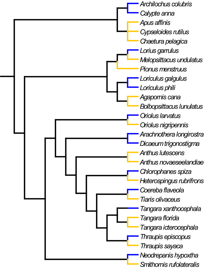
Figure 1. Phylogenetic relationships of species sequenced. Blue and orange branches indicate nectarivores and non-nectarivores respectively. Branch lengths are not to scale. Tree was produced using Mesquite Version 3.61. (Maddison and Maddison 2019) and published phylogenies (Burns et al. 2003; Warren et al. 2006; Zhang et al. 2007; Hackett et al. 2008; Irestedt and Ohlson 2008; Wright et al. 2008; Hedges and Kumar 2009; Reding et al. 2009; Weir et al. 2009; Jønsson et al. 2010; Sedano and Burns 2010; Moyle et al. 2011; Jetz et al. 2012)
Table 1 Representative species from divergent taxa of nectarivorous (with double asterisks) and non-nectarivorous (without asterisks) diet used in this study
Contrast Clades compared Sequenced representatives of each contrast Common name 1 Lorikeets and budgerigars and an outgroup Lorius garrulus (nectarivore)** Chattering Lorry Melopsittacus undulatus (non-nectarivore) Budgerigar Pionus menstruus (non-nectarivore) Blue-headed Parrot 2 Sunbird-asities and broadbills Neodrepanis hypoxtha (nectarivore)** Yellow-bellied Sunbird-asity Smithornis rufolateralis (non-nectarivore) Rufous-sided Broadbill 3 Hanging parrots and lovebirds/guaiaberos Loriculus galgulus (nectarivore)** Blue-crowned Hanging Parrot Loriculus phili (nectarivore)** Philippine Hanging Parrot Agapornis cana (non-nectarivore) Grey-headed Lovebird Bolbopsittacus lunulatus (non-nectarivore) Guaiabero 4 Hummingbirds and swifts Calypte anna (nectarivore)** Anna's Hummingbird Archilochus colubris (nectarivore)** Ruby-throated Hummingbird Apus affinis (non-nectarivore) House Swift Cypseloides rutilus (non-nectarivore) Chestnut-collared Swift Chaetura pelagica (non-nectarivore) Chimney Swift 5 Saffron-crowned tanager and related tanagers Tangara xanthocephala (nectarivore)** Saffron-crowned Tanager Tangara florida (non-nectarivore) Emerald Tanager Tangara icterocephala (non-nectarivore) Silver-throated Tanager 6 Flowerpeckers/sunbirds and motacillidae Arachnothera longirostra (nectarivore)** Little Spiderhunter Dicaeum trigonostigma (nectarivore)** Orange-bellied Flowerpecker Anthus lutescens (non-nectarivore) Yellowish Pipit Anthus novaeseelandiae (non-nectarivore) Newzealand Pipit 7 Green Honeycreeper and related tanagers Chlorophanes spiza (nectarivore)** Green Honeycreeper Heterospingus rubrifrons (non-nectarivore) Sulphur-rumped Tanager 8 O. larvatus and O. nigripennis Oriolus larvatus (non-nectarivore)** Black-headed Oriole Oriolus nigripennis (nectarivore) Black-winged Oriole 9 T. episcopus and T. sayaca Thraupis episcopus (nectarivore)** Blue-gray Tanager Thraupis sayaca (non-nectarivore) Sayaca Tanager 10 Banaquits and grassquits Coereba flaveola (nectarivore)** Bananquit Tiaris olivaceus (non-nectarivore) Yellow-faced Grassquit Arbitrary numbers are assigned to each contrast and dietary category is indicated  下载: 导出CSV
-
-
期刊类型引用(3)
1. Dey, P., Ray, S.D., Kochiganti, V.H.S. et al. Mitogenomic Insights into the Evolution, Divergence Time, and Ancestral Ranges of Coturnix Quails. Genes, 2024, 15(6): 742.  必应学术
必应学术
2. Fuentes-López, A., Rebelo, M.T., Romera, E. et al. Genetic diversity of Calliphora vicina (Diptera: Calliphoridae) in the Iberian Peninsula based on cox1, 16S and ITS2 sequences. Biological Journal of the Linnean Society, 2020, 131(4): 952-965. 必应学术
3. Chen, Y.. Does the diversification rate of endemic birds of mainland China follow abrupt, gradual shifting or constant patterns?. Integrative Zoology, 2017, 12(2): 165-171. 必应学术
其他类型引用(0)